

Why Normalize?
Sometimes, a database design that looks OK at first sight may have some hidden problems. One such kind of problem is Non-Atomic values. This means that the value stored in a single column in the database is actually a combination of multiple values which makes the database harder to work with because you’ll always need expressions to extract the individual value. And it comes with major impact to the performance as well.
- Non-Atomic Values
- Complex Code Required
- Performance Impact
A database design suffers from redundancy if it allows multiple copies of the same fact (data) to be stored, which is bad for several reasons, as mentioned below -
- Same data is stored multiple places
- Storage space is wasted
- Performance Impact
- The possibility of Conflicting Data (Data Inconsistency)
The third problem that may harm in the database is Modification Anomalies.
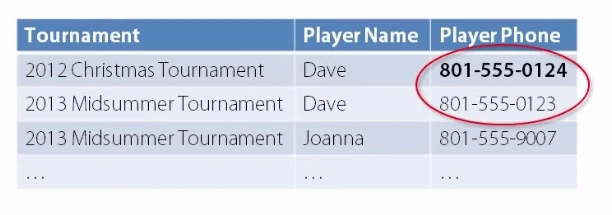
Suppose Dave wants to update the Phone Number; then we update it in the first place. So, we also need to update it in other places as well. This is an Update Anomaly.
Let’s suppose Joanna doesn’t want to participate in the tournament. So, we delete the 3rd record (Joanna) from the table which means we lost the other information as well like Joanna's Phone Number etc. This is Delete Anomaly.
In order to resolve such kind of issues, we have to normalize our database. So, here, we have a few steps which we call as Normal Forms.
- First Normal Form (1NF)
- Second Normal Form (2NF)
- Third Normal Form (3NF)
- Elementary Key Normal Form (EKNF)
- Boyce-Codd Normal Form (BCNF)
- Fourth Normal Form (4NF)
- Fifth Normal Form (5NF)
- Domain/Key Normal Form (DKNF)
- Sixth Normal Form (6NF)
These normal forms always apply to an individual table. So within the single database or a single relational data model, some tables may be fourth or fifth normal form others may be on the 3rd normal form. Everyone agrees that the table should be normalized at the 3rd normal form at a minimum but here, we have different opinions as well.
When people mention the normal form of the design or of the database, they actually mean the lowest normal form of all its tables. Let’s say a database has 20 tables at the 5th normal form, 3 tables on 4th normal form, and 1 table on the 2nd normal form. We would say the database is in 2nd normal form.
Many people normalize their design after converting their Entity-Relationship model to Relational Database. However, because the ER diagram is the logical documentation this means that any changes made to the relational database design as a result of normalization should be ported back to ER model as well.
- Most Common Approach
- Convert Entity-Relationship Model to Relational Tables
- Normalize Relational Tables
- Disadvantage - Changes must be ported back to ER Model
- Alternative Approach
- Normalize the ER Model
- Convert Normalized ER model to Relational Tables
- Disadvantage - Normalization is Bit More Complicated
When We Should Normalize Our Database
We’re studying Normalization from the very beginning of our engineering which shows how important it is, like the essential part of the database. Which is wrong. If you have made your application's database with just your understanding, then it will be ok. But if you have applied Normalization Rules to make it normalize then we’ll make our database consistent of data and we can remove the repetition of data on multiple places. It was just a general point of discussion. Now let’s discuss technically where we really need to implement Normalization.
Applications are of 2 types.
- OLTP (Online Transaction Processing)
This kind of application can have hundreds and thousands of transactions in a day. Most of the time we’re implementing insertion, updation, deletion and reading the records of a specific member. In such a database, we should normalize our model, which makes our data less redundant, more accurate and more inconsistent. Here our customers' data is very important, so we take much care of the data.
- OLAP (Online Analytics Processing)
In OLAP applications, we mostly perform reporting. We use this model to implement the forecasting from the previous history of the data. Most of the time we just implement the read operation here. So in such a scenario, our denormalized database is OK.
To understand both of the above opinions, let me explain the reason. Actually when we normalize the table, we divide it into sub-multiple tables and when we cut the tables into pieces and again try to retrieve the records from these tables we need to implement a lot of joins to get the data and sometimes the query becomes more complex in these joins which affects our database performance with respect to the speed of database results back. But in OLAP, if we don’t normalize our tables, our tables are in their original form containing a lot of redundant data but here we don't have any chunks of small pieces of tables. So here we directly just select the records and display it on the screen which will be very fast in the denormalized state.
Now you can easily make the decision, when to normalize the database and when we should not.
Note
To implement the Normalization in the database, there are 2 important things. You should have the knowledge of Functional Dependency and you should have the knowledge of Keys. Without this prior knowledge, you can’t implement the Normalization in the database.
Functional Dependency
A functional dependency is a relationship between 2 or more attributes. It means if the value of one attribute is known, it is possible to obtain the value of another attribute.
Suppose there is a relation STUDENT with following fields:
STUDENT (RegistrationNo, StudentName, Class, Email)
If the value of RegistrationNo is known, it is possible to obtain the value of StudentName. It means that StudentName is functionally dependent upon RegistrationNo. An attribute B is functionally dependent on A if the value of A determines the value of B.
Functional Dependency is written as follows,
RegistrationNo --> StudentName
An attribute can also functionally dependent upon two or more attributes instead of a single attribute.
COURSE(STUDID, CRSNO, CRSDATE)
The attribute CRSDATE is functionally dependent on both STUDID and CRSNO in the above example.
The functional dependency in the relation is represented as,
STUDID, CRSNO --> CRSDATE
So here course completion date CRSDATE can be determined only if both STUDID and CRSNO are known. No single attribute can be used to determined CRSDATE.
In Mathematics, the relationship between variables is called a function. And functional dependency is when some attributes are dependent upon some other attributes. There are 2 types of functional dependency.
Suppose A, B, and C are the attributes (columns) of a table.
- Trivial Dependency
Let’s discuss this type with example. Suppose,
AB --> A
Suppose A and B are 2 columns of a table. And with the help of A and B we’re not getting any new value back which means even the combination of 2 columns in a table don’t identify the new record values.
- Non-Trivial Dependency
Non-Trivial dependency gives us different values in response.
AB --> C
And here A and B are 2 columns of a table and A & B pointing to a unique record and gives us the new value in response which is C.
This is the general concept of functional dependency.
Keys
Now let’s discuss the concept of keys. Suppose,
R (ABCD)
Here R is a table containing 4 columns. Now the functional dependency in this relation is,
A --> BC
Which means if we have the value of A we can conclude the values of BC columns as well. Columns B and C depend upon the column A. So what would you say, Can we use A as the key here? Absolutely No, because the key in a table is which identifies our all the records in a table.
Now, let’s suppose we have some more dependencies.
ABC --> D, AB --> CD, A --> BCD
- In the first dependency (ABC --> D), D depends upon ABC. We have already ABC and with the help of ABC, we can get D. So now we have ABCD which means our table is completed. So, we can use ABC as a key.
- Similarly, in the 2nd dependency (AB --> CD), CD depends upon AB. We have already AB and we can conclude CD in response. So we can also use AB as a key.
- Now the 3rd functional dependency is (A --> BCD). So with the help of only A, we can get all the remaining columns of the table. So we can also use A as a key.
This key is called Super Key. Once again, a Super key is the key with the help of which we can uniquely identify a row or a tuple in a table or we can uniquely identify all the remaining attributes of the table.
(S.K)+ = R
Now let’s suppose you’re a Database Administrator. Just ask yourself, what key you’ll use in your table among these dependencies?
ABC --> D, AB --> CD, A --> BCD
Now obviously we’ll use (A --> BCD) because it is more efficient than all the dependencies and it is uniquely identifying the complete record. So A is the Candidate Key. Candidate Key is actually the most efficient version of Super Keys and in our remaining dependencies (ABC & AB) are just the SuperKeys only.
Now let’s see another example, let’s suppose
R (ABCD) & B --> ACD, ACD --> B
So in the first functional dependency, we can get all the remaining attributes of a table from B column. So B is the Super Key.
In the second dependency (ACD --> B), we have already ACD and with the help of ACD, we can get the value of B because B is dependent upon ACD. So ACD is also a Super Key.
Now, what about Candidate Keys?
B is also a Candidate Key because it is very efficient and helps us to identify all the remaining attributes of a column.
ACD is also a Candidate Key because with the help of ACD we can get the value of B and our table will become complete. So ACD is also a Candidate Key.
Now it is the time of Primary Key.
Now you can see we have 2 candidate keys in a table.
R (ABCD) & B --> ACD, ACD --> B
Now we can think about the functional dependency in the relation which is more efficient. Obviously, we’ll say B is a more efficient candidate key. So Database Administrator will make B as a primary key in the table which will point to all the remaining data in the table. And if he chooses B as the primary key then ACD will become our Alternate Key.
And sometimes to find the B is quite critical. Let me explain, suppose you have purchased something online. The transaction is generated and the amount is deducted from your account but you didn’t get the things. Now you make the call to the helpline of that company, he asks you the transaction id of your transaction. Of course transaction id is the primary key in his system database but now you don’t remember the transaction id. Then he asks you please tell us when you purchase the products (Date Timing), what’s your name? What are the products you purchased? Now with the help of this information, he can easily find your record in his system. So don’t think always B is the best option for the primary key, we should also think about the different real-world scenarios as well.
When you make the primary key with the help of 1+ attributes, it will become the composite key of the table.
An attribute or set of attributes that is the basis for data retrieval is known as a secondary key. It can be a non-unique attribute. One secondary key value may refer to many records. For example, an attribute Address in Student table can be used to display all students who live in a particular city. In this case, Address will be used as a secondary key.
First Normal Form
A relationship is in 1NF if every intersection of row and column contains atomic values only. It means that the relation doesn’t contain any repeating group. A repeating group is a set of one or more data items that may occur a variable number of times in a tuple. Each cell in a relationship should contain only one variable.
A relation can be converted into 1NF using two methods,
- Method 1
In this method, the repeating groups are removed by entering proper data in blank fields that contain repeating data.
- Method 2
In this method, we create a new relation to removing the repeating groups. The repeating data is stored in the new relation.
Example
Suppose we have the following un-normalized relation DEPARTMENT,
DEPARTMENT(Dept_No, Dept_Name, Emp_No, Emp_Name)
Suppose the data in the relation is as follows,
| Dept_No | Dept_Name | Emp_No | Emp_Name |
| 10 | Management | E01E02 | Usman Khalil Abdullah |
| 20 | Finance | E10E11 | Ali AhmadMahmood Abbas |
| 30 | IT | E25 | Hamid Ali |
Applying Method 1
The above relation contains the repeating groups. The attributes Emp_No and Emp_Name are being repeated for a single occurrence of Dept_No. The repeating groups are removed by entering proper data in the blank fields as follows.
| Dept_No | Dept_Name | Emp_No | Emp_Name |
| 10 | Management | E01 | Usman Khalil |
| 10 | Management | E02 | Abdullah |
| 20 | Finance | E10 | Ali Ahmad |
| 20 | Finance | E11 | Mahmood Abbas |
| 30 | IT | E25 | Hamid Ali |
The above relation is now in 1NF as each field contains a single value. It will have a composite key that consists of Dept_No and Emp_No attributes.
Applying Method 2
The second method to remove the repeating groups and make the cells atomic is by creating a new relation. It means the above un-normalized table will be divided into 2 relations. And then we’ll make the relationship between these two tables.
| Dept_No | Dept_Name |
| 10 | Management |
| 20 | Finance |
| 30 | IT |
Department
| Dept_No | Emp_No | Emp_Name |
| 10 | E01 | Usman Khalil |
| 10 | E02 | Abdullah |
| 20 | E10 | Ali Ahmed |
| 20 | E11 | Mahmood Abbas |
| 30 | E25 | Hamid Ali |
Employee
Hard and Fast Rule of Relationship Among Tables
So the hard and fast rule is we always declare the foreign key attribute in the table which is dependent, which is the child of any parent table. And now here in our scenario Employee can’t exist if there is no department in any organization. Department can exist without Employee but Employee can’t exist without Department. So Department is the parent table and Employee is the child table. So the relationship will be 1:M from Department to Employee and if we’re interested to know the relation from the right side than obviously the relationship from Employee to Department is 1:1
A type of dependency in which one or more non-key attributes are functionally dependent on a part of the primary key is called partial dependency.
Example
Student(Stud_Id, Name, Dept, MonFee, CRSNo, CRSDT)
The relation contains a composite primary key that consists of Stud_Id, and CRSNo.
| Stud_Id | Name | Dept | MonFee | CRSNo | CRSDT |
| 100 | Ahmad | Marketing | 1000 | SPSS | 19/06/96 |
| 100 | Ahmad | Marketing | 1000 | SURVEYS | 10/07/96 |
| 140 | Nazir | Accounting | 1200 | TAXACCT | 12/08/97 |
| 110 | Hamid | Info. System | 1100 | SPSS | 14/07/96 |
| 110 | Hamid | Info. System | 1100 | COBOL | 22/07/96 |
| 190 | Rashid | Finance | 1200 | INVESTMENT | 20/07/96 |
| 150 | Hussain | Marketing | 1000 | SPSS | 19/06/98 |
| 150 | Hussain | Marketing | 1000 | SYSANAL | 20/07/98 |
Student
The financial dependencies in this relation are as follows:
The non-key attributes Name, Dept, MonFee are functionally dependent on a part of primary key Stud_Id. They are not functionally dependent on a complete key. It is called partial dependency. The partial dependency in the above relation creates redundancy. It results in certain database anomalies when the relation is updated.
Problem with Partial Dependency
We already know that the primary key can’t be null. But if we make the primary key with the help of a composite key, then for the primary key condition if any attribute has the value and the next attribute is null then it is ok for the primary key. Like,
(Stud_Id + CRSNo) is the primary key. But if CRSNo is null but Stud_Id has some value then it is ok primary key.
Now look above functional dependency,
Stud_Id --> Name, Dept, MonFee
Stud_Id, CRSNo --> CRSDT
Look CRSDT is an advantage because it is dependent upon Stud_Id and CRSNo. So if any attribute Stud_Id or CRSNo becomes null then we can even find CRSDT. But if you see the first functional dependency.
Stud_Id --> Name, Dept, MonFee
All these 3 attributes depend only on Stud_Id. And if Stud_Id becomes null then from Stud_Id we can’t compute these 3 attributes.
Now, remember the definition of the Super Key is we can find the complete relationship with the help of this key. This primary key can identify the complete row of data. But in this our case, our promise doesn’t hold because the primary key is valid if any attribute in the composite key is null. And if Stud_Id is null then we can’t compute the values of Name, Dept, MonFee.
Insertion Anomaly
Suppose a new course WEBDEV is to be inserted in the relation. The new CRSNo cannot be inserted in the relation without inserting Stud_Id. The primary key consists of Stud_Id and CRSNo.
Deletion Anomaly
Similarly suppose we want to delete the record of 190 Stud_Id and if you try to delete this record, obviously you’ll lose Course information as well. INVESTMENT CRSNo will automatically delete with Stud_Id record.
Second Normal Form
A relation is in 2NF if it is in the 1NF and every non-key attribute is fully functionally dependent on the primary key. All non-key attributes must depend on all parts of the primary key. If the table has just only 1 attribute for the primary key then obviously it will be in 2NF automatically because partial dependency doesn’t exist here.
Most of the time we create the relation of each entity. It will make our work a lot easier. The conditions of 1NF are,
The primary key should contain one attribute. It doesn’t mean that we can’t create the composite primary key in the table to satisfy it for the 2NF. Yes, we can create the composite primary key but make sure that all the non-key attributes are fully dependent upon both composite primary key.
- Stud_Id --> Name, Dept, MonFee
- Stud_Id, CRSNo --> CRSDT
This kind of dependency on the table makes the problem and here we’re not satisfying the 2NF. But if the scenario is,
Stud_Id, CRSNo --> Name, Dept, MonFee, CRSDT
Now it is ok because every non-key attribute is fully functionally dependent on the full set of primary key.
Now let’s make our Student relation satisfy for the 2NF. So what will we do?
All the partially dependent attributes should be removed and place in another relation. So,
Student1(Stud_Id, Name, Dept, MonFee)
| Stud_Id | Name | Dept | MonFee |
| 100 | Ahmad | Marketing | 1000 |
| 100 | Ahmad | Marketing | 1000 |
| 140 | Nazir | Accounting | 1200 |
| 110 | Hamid | Info. System | 1100 |
| 110 | Hamid | Info. System | 1100 |
| 190 | Rashid | Finance | 1200 |
| 150 | Hussain | Marketing | 1000 |
| 150 | Hussain | Marketing | 1000 |
Student1
Course(Stud_Id, CRSNo, CRSDT)
| Stud_Id | CRSNo | CRSDT |
| 100 | SPSS | 19/06/96 |
| 100 | SURVEYS | 10/07/96 |
| 140 | TAXACCT | 12/08/97 |
| 110 | SPSS | 14/07/96 |
| 110 | COBOL | 22/07/96 |
| 190 | INVESTMENT | 20/07/96 |
| 150 | SPSS | 19/06/98 |
| 150 | SYSANAL | 20/07/98 |
Course
And in the Course relation, we’re making the 2 attributes as a primary key. And our problem is solved. Now the table is in the 2NF.
A transitive dependency is a type of functional dependency between 2 or more non-key attributes. It exists if a non-key attribute depends upon any other non-key attribute. It means the value of a non-key attribute can be obtained by knowing the value of another non-key attribute.
| CUSTNO | NAME | SALESMAN | REGION |
| 10 | Ahsan | Ahmad | South |
| 20 | Babar | Bashir | West |
| 30 | Chauhan | Ahmad | South |
| 40 | Daood | Khalid | East |
| 50 | Ehtasham | Bashir | West |
| 60 | Farooq | Munir | North |
Sales
The above relation contains the following functional dependencies,
- CUSTNO --> NAME, SALESMAN
- SALESMAN --> REGION
The above relation fulfills the 2NF because the primary key consists of a single attribute. A transitive dependency exists in the relation. The REGION is functionally dependent on SALESMAN and SALESMAN is functionally dependent on CUSTNO. It means that REGION is transitive dependent on CUSTNO.
The transitive dependency creates the following anomalies.
Insertion Anomaly
The insertion anomaly occurs when a new record is inserted in the relation. Suppose a new salesman “Abid” joins the company and is assigned to North region. The record of the new salesman cannot be entered until a customer is also assigned to him because the primary key of the relation is CUSTNO.
Deletion Anomaly
The deletion anomaly occurs when a record is deleted from the relation. Suppose the record of CUSTNO 40 is to be deleted. It will also delete the information of the salesman “Khalid” who is assigned to East.
Third Normal Form
The relation is in the 3NF if it is in the 2NF and no transitive dependency exists. The transitive dependency is an important factor in normalization. A relation is not in 3NF if the value of non-key attributes can be obtained by knowing the value of another non-key attribute.
Removing Transitive Dependency
Any transitive dependencies are removed to convert a relation from 2NF to 3NF. The above anomalies occur due to transitive dependency. The transitive dependency can be removed by decomposing the above relation into two relations as follows:
| CUSTNO | NAME | SALESMAN |
| 10 | Ahsan | Ahmad |
| 20 | Babar | Bashir |
| 30 | Chauhan | Ahmad |
| 40 | Daood | Khalid |
| 50 | Ehtasham | Bashir |
| 60 | Farooq | Munir |
Sales1
| SALESMAN | REGION |
| Ahmad | South |
| Bashir | West |
| Khalid | East |
| Munir | North |
Salesman
Conclusion
Up to 3NF our database is actually ready for the OLTP databases. And if we go further then obviously we’ll need to break the table into sub-tables. And that is not good, because we need to create a lot of joins to get the data and our queries will become complex. So most of the time you’ll see normal forms at 3 level.
Abhishek MishraPosted Oct 5, 2018, 4:07 AM
Very well articulated