KNN- K-Nearest Neighbors using Python

K Nearest Neighbor using Python

In the previous article, we studied the Naive Bayes. One thing that I believe is that if we can correlate anything with us or our lives, there are greater chances of understanding the concept. So I will try to explain everything by relating it to humans.

What is K nearest neighbor used for?

KNN can be used for both classification and regression predictive problems. However, it is more widely used in classification problems in the industry. k-NN is often used in search applications where you are looking for “similar” items; that is when your task is some form of “find items similar to this one”. We use k-NN when we have fewer than 20 features (attributes) per instance, typically normalized or we have a lot of training data.

What is KNN?

KNN is a non-parametric, lazy learning algorithm; i.e. it does not make any assumptions on the underlying data and also there is no explicit training phase or it is very minimal.

k-NN is all about finding the next data point(s) which is at the minimum distance from the current data point and to club all into one class.

k is the max value of data point(s) that can be clubbed under a given class.

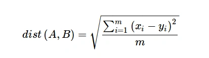
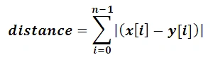
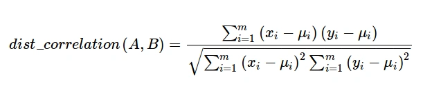
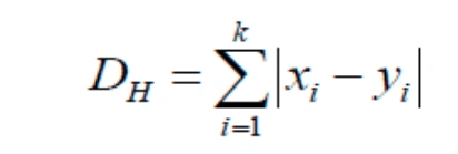
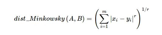
To find the distance we use employ various algorithms like Euclidean Distance, Hamming Distance, Manhattan Distance, Minkowski Distance, etc.

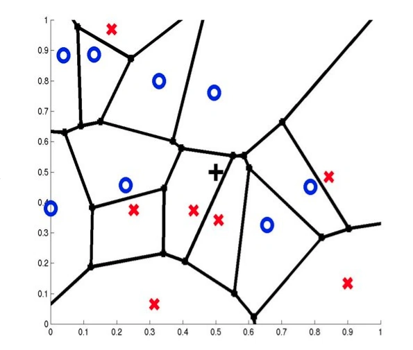
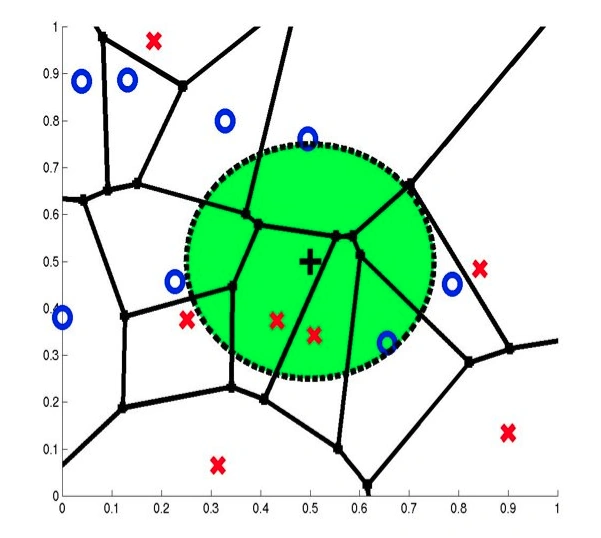
For example, 1-NN means that we have to generate a model that will have classes based on the data point which is at the least distance. Similarily, 2-NN means that we have to generate a model that will have classes based on the 2 data points with the least distances.

The algorithm of k-NN or K-Nearest Neighbors is:

Computes the distance between the new data point with every training example.
For computing, distance measures such as Euclidean distance, Hamming distance or Manhattan distance will be used.
The model picks K entries in the database which are closest to the new data point.
Then it does the majority vote i.e the most common class/label among those K entries will be the class of the new data point.

Steps involved in the processing and generating a model

Decide on your similarity or distance metric.
Split the original labeled dataset into training and test data.
Pick an evaluation metric.
Decide upon the value of k. Here k refers to the number of closest neighbors we will consider while doing the majority voting of target labels.
Run k-NN a few times, changing k and checking the evaluation measure.
In each iteration, k neighbors vote, majority vote wins and becomes the ultimate prediction
Optimize k by picking the one with the best evaluation measure.
Once you’ve chosen k, use the same training set and now create a new test set with the people’s wages and incomes that you have no labels for, and want to predict.

Steps involved in selecting the value for K

Determined experimentally
Start with k=1 and use a test set to validate the error rate of the classifier
Repeat with k=k+2
Choose the value of k for which the error rate is minimum
Note: k should be an odd number to avoid ties

1-NN

3-NN

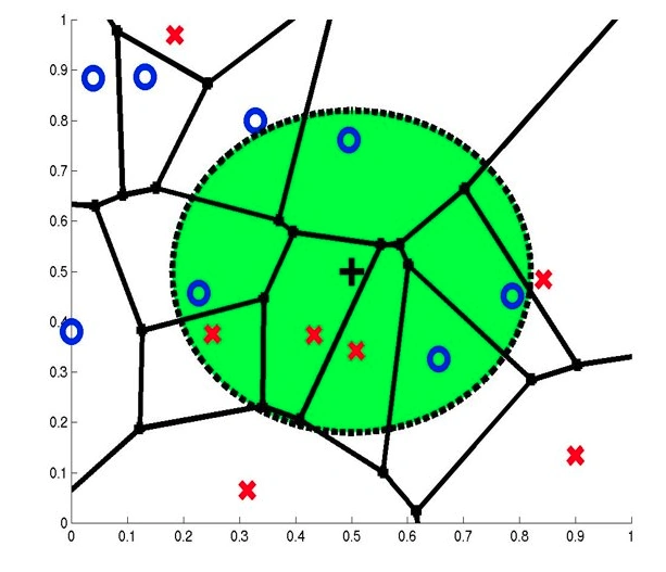
7-NN

KNN vs K-Means Clustering

	k-NN	k-Means
Types	Supervised	Unsupervised
What is K?	Number of closest neighbors to look at	Number of centroids
Calculation of prediction error possible	Yes	No
Optimization is done using what?	Cross-validation and confusion matrix	Elbow method and the silhouette method
Algorithm convergences	When all observations classified at the desired accuracy	When cluster membership doesn't change anymore
Complexity	Training: O(Dimensions/Features) Test: O (Number of Observations)	O (Number of points * Number of Clusters * Number of iterations * number of attributes)

Curse of Dimensionality

Imagine instances described by 20 features (attributes) but only 3 are relevant to the target function. Curse of dimensionality means that nearest neighbor can be easily misled when instance space is high-dimensional and is dominated by a large number of irrelevant features.

A solution to this can be

Stretch j-th axis by weight zj, where z1,…,zn chosen to minimize prediction error (weight different features differently)
Use cross-validation to automatically choose weights z1,…,zn
Note setting zj to zero eliminates this dimension altogether (feature subset selection)
PCA

Advantages/Features of KNN

K-NN is pretty intuitive and simple
The K-NN algorithm is easy to implement and very simple to understand. It reads through the whole dataset to classify the new data point and to find out K nearest neighbors.
K-NN has fewer assumptions
K-NN is a non-parametric algorithm which means there are fewer assumptions to be met to implement K-NN. Parametric models like linear regression have lots of assumptions to be met by data before it can be implemented which is not the case with K-NN.
No Training Step
K-NN does not explicitly build any model and simply tags the new data entry based learning from historical data, hence no training step is required.
It constantly evolves
The classifier immediately adapts as we collect new training data and respond quickly to changes in the input during real-time use.
Very easy to implement for the multi-class problem
K-NN adjusts to multi-class without any extra efforts as compared to other algorithms.
Can be used both for Classification and Regression
One of the biggest advantages of K-NN is that K-NN can be used both for classification and regression problems.
One Hyper Parameter
K-NN might take some time while selecting the first hyperparameter but after that rest of the parameters are aligned to it.
KNN stores the entire training dataset which it uses as its representation.
KNN does not learn any model.
KNN makes predictions just-in-time by calculating the similarity between an input sample and each training instance.
A variety of distance criteria to choose from the K-NN algorithm gives the user the flexibility to choose distance while building a K-NN model.
- Euclidean Distance
- Hamming Distance
- Manhattan Distance
- Minkowski Distance

Disadvantages/Shortcomings of KNN

K-NN is a slow algorithm
K-NN might be very easy to implement except for the fact that as the dataset grows efficiency/speed of algorithm declines very fast.
Curse of Dimensionality
KNN predicting efficiency decreases as the numbers of variables grow works.
K-NN needs homogeneous features
If you decide to build k-NN using a common distance, like Euclidean or Manhattan distances, it is completely necessary that features have the same scale, since absolute differences in features weight the same, i.e., a given distance in feature 1 must mean the same for feature 2.
An optimal number of neighbors
One of the biggest and most crucial issues with K-NN is to choose the optimal number of neighbors to be considered while classifying the new data entry.
Imbalanced data causes problems
k-NN doesn’t perform well on imbalanced data.
Outlier sensitivity
K-NN algorithm is very sensitive to outliers as it simply chose the neighbors based on distance criteria.
Missing Value treatment
K-NN inherently has no capability of dealing with missing value problems.

Assumptions of KNN

k-NN performs much better if all of the data have the same scale
k-NN works well with a small number of input variables (p) but struggles when the number of inputs is very large
k-NN makes no assumptions about the functional form of the problem is solved

Euclidean distance

Manhattan Distance

Chi-Square Distance

Correlation Distance

Hamming Distance

Minkowsky Distance

KNN using an example

Let us understand how k-NN really works. For that let's take a dummy dataset.

data = [
[65.75, 112.99],
[71.52, 136.49],
[69.40, 153.03],
[68.22, 142.34],
[67.79, 144.30],
[68.70, 123.30],
[69.80, 141.49],
[70.01, 136.46],
[67.90, 112.37],
[66.49, 127.45],
]

In the above example, the data is of the form [feature, target].

Assuming the value of k to be 3 i.e. 3-NN, let's try to find the prediction for feature value "60".

So the 3 nearest neighbors would be

a. 65.75 with a distance value 5.75

b. 66.49 with a distance value 6.49

c. 67.79 with a distance value 7.79

And hence the predicted value will be 128.25.

Similarly, let's take another dataset

data = [
[22, 1],
[23, 1],
[21, 1],
[18, 1],
[19, 1],
[25, 0],
[27, 0],
[29, 0],
[31, 0],
[45, 0],
]

In the above example, the data is of the form [feature, target].

Assuming the value of k to be 3 i.e. 3-NN, let's try to find the prediction for feature value "33".

So the 3 nearest neighbors would be

a. 31 with a distance value 2.0

b. 29 with a distance value 4.0

c. 27 with a distance value 6.0

And hence the predicted value will be 0.

Python Implementation of Decision Tree

Let's take the example of the MNIST dataset, you can directly import it from the sklearn dataset repository or download it from the article. Feel free to use any dataset, there are some very good datasets available on kaggle and with Google Colab.

Before we start with this, it is highly recommended you read the following tutorials

1. From Scratch

Here, I will be using some dummy data. You can use and practice on any kind of data

from collections import Counter
import math

In the above code, we are exporting the required libraries.

def knn(data, query, k, distance_fn, choice_fn):
neighbor_distances_and_indices = []
# 3. For each example in the data
for index, example in enumerate(data):
# 3.1 Calculate the distance between the query example and the current
# example from the data.
distance = distance_fn(example[:-1], query)
# 3.2 Add the distance and the index of the example to an ordered collection
neighbor_distances_and_indices.append((distance, index))
# 4. Sort the ordered collection of distances and indices from
# smallest to largest (in ascending order) by the distances
sorted_neighbor_distances_and_indices = sorted(neighbor_distances_and_indices)
# 5. Pick the first K entries from the sorted collection
k_nearest_distances_and_indices = sorted_neighbor_distances_and_indices[:k]
# 6. Get the labels of the selected K entries
k_nearest_labels = [data[i][1] for distance, i in k_nearest_distances_and_indices]
# 7. If regression (choice_fn = mean), return the average of the K labels
# 8. If classification (choice_fn = mode), return the mode of the K labels
return k_nearest_distances_and_indices , choice_fn(k_nearest_labels)

In the above code, we have created a function that will perform all the required tasks to result out a k-NN based model

#function to calculate the mean used in case of regression
def mean(labels):
return sum(labels) / len(labels)
#function to calculate the mode used in case of classification
def mode(labels):
return Counter(labels).most_common(1)[0][0]
#function to calculate the distance between two data points
def euclidean_distance(point1, point2):
sum_squared_distance = 0
for i in range(len(point1)):
sum_squared_distance += math.pow(point1[i] - point2[i], 2)
return math.sqrt(sum_squared_distance)

The above code lists down all the auxiliary functions used during the program

# Regression Data
#
# Column 0: height (inches)
# Column 1: weight (pounds)
'''
reg_data = [
[65.75, 112.99],
[71.52, 136.49],
[69.40, 153.03],
[68.22, 142.34],
[67.79, 144.30],
[68.70, 123.30],
[69.80, 141.49],
[70.01, 136.46],
[67.90, 112.37],
[66.49, 127.45],
]

The above code, declares the dummy regression data, in the above data column 0 signifies height and column 1 signifies weight

reg_query = [60]
reg_k_nearest_neighbors, reg_prediction = knn(
reg_data, reg_query, k=3, distance_fn=euclidean_distance, choice_fn=mean
)
print(reg_k_nearest_neighbors, reg_prediction)

In the above code, we will generate a model, and then based on that model will predict the weight for a person with a height of 60

'''''''
# Classification Data
#
# Column 0: age
# Column 1: likes pineapple
'''
clf_data = [
[22, 1],
[23, 1],
[21, 1],
[18, 1],
[19, 1],
[25, 0],
[27, 0],
[29, 0],
[31, 0],
[45, 0],
]

The above code, declares the dummy data for classification based problem, where column 0 signifies age and column 1 signifies if a person like pineapple or not

clf_query = [33]
clf_k_nearest_neighbors, clf_prediction = knn(
clf_data, clf_query, k=3, distance_fn=euclidean_distance,choice_fn=mode)
print(clf_k_nearest_neighbors, clf_prediction)

In the above code, we first create a model and based on that model, we predict if a 33 years old person likes pineapple or not.

scratch_knn.py

from collections import Counter
import math
def knn(data, query, k, distance_fn, choice_fn):
neighbor_distances_and_indices = []
# 3. For each example in the data
for index, example in enumerate(data):
# 3.1 Calculate the distance between the query example and the current
# example from the data.
distance = distance_fn(example[:-1], query)
# 3.2 Add the distance and the index of the example to an ordered collection
neighbor_distances_and_indices.append((distance, index))
# 4. Sort the ordered collection of distances and indices from
# smallest to largest (in ascending order) by the distances
sorted_neighbor_distances_and_indices = sorted(neighbor_distances_and_indices)
# 5. Pick the first K entries from the sorted collection
k_nearest_distances_and_indices = sorted_neighbor_distances_and_indices[:k]
# 6. Get the labels of the selected K entries
k_nearest_labels = [data[i][1] for distance, i in k_nearest_distances_and_indices]
# 7. If regression (choice_fn = mean), return the average of the K labels
# 8. If classification (choice_fn = mode), return the mode of the K labels
return k_nearest_distances_and_indices , choice_fn(k_nearest_labels)
def mean(labels):
return sum(labels) / len(labels)
def mode(labels):
return Counter(labels).most_common(1)[0][0]
def euclidean_distance(point1, point2):
sum_squared_distance = 0
for i in range(len(point1)):
sum_squared_distance += math.pow(point1[i] - point2[i], 2)
return math.sqrt(sum_squared_distance)
def main():
'''''
# Regression Data
#
# Column 0: height (inches)
# Column 1: weight (pounds)
'''
reg_data = [
[65.75, 112.99],
[71.52, 136.49],
[69.40, 153.03],
[68.22, 142.34],
[67.79, 144.30],
[68.70, 123.30],
[69.80, 141.49],
[70.01, 136.46],
[67.90, 112.37],
[66.49, 127.45],
]
# Question:
# Given the data we have, what's the best-guess at someone's weight if they are 60 inches tall?
reg_query = [60]
reg_k_nearest_neighbors, reg_prediction = knn(
reg_data, reg_query, k=3, distance_fn=euclidean_distance, choice_fn=mean
)
print(reg_k_nearest_neighbors, reg_prediction)
'''''
# Classification Data
#
# Column 0: age
# Column 1: likes pineapple
'''
clf_data = [
[22, 1],
[23, 1],
[21, 1],
[18, 1],
[19, 1],
[25, 0],
[27, 0],
[29, 0],
[31, 0],
[45, 0],
]
# Question:
# Given the data we have, does a 33 year old like pineapples on their pizza?
clf_query = [33]
clf_k_nearest_neighbors, clf_prediction = knn(
clf_data, clf_query, k=3, distance_fn=euclidean_distance, choice_fn=mode
)
print(clf_k_nearest_neighbors, clf_prediction)
if __name__ == '__main__':
main()

The output that I got is:

Regression case:

Neighbors: [(5.75, 0), (6.489999999999995, 9), (7.790000000000006, 4)]

Prediction: 128.24666666666667

Classification case:
Neighbors: [(2.0, 8), (4.0, 7), (6.0, 6)]

Prediction: 0

2. Using SkLearn

In sklean, we have KNeighnotsClassifier class, used for implementing k-NN

knn_sklearn.py

X = [[0], [1], [2], [3]]
y = [0, 0, 1, 1]
from sklearn.neighbors import KNeighborsClassifier
neigh = KNeighborsClassifier(n_neighbors=2)
neigh.fit(X, y)
print(neigh.predict([[4.567]]))
print(neigh.predict_proba([[4.567]]))

In the above code, we create a dummy data, which is then passed to the classifier, to get the predicted value and predicting probability corresponding to 4.567

The output that I got is

Predicted value: [1]
Predicting Probability: [[0. 1.]]

3. Using TensorFlow

Here I will be using the MNSIT cloth dataset.

from __future__ import print_function
import numpy as np
import tensorflow as tf

In the above code, we are importing all the required libraries.

In the below code, I have commented on Line numbers 41 and 42, you can uncomment those if you want to see the complete output.

knn_tensorflow.py

from __future__ import print_function
import numpy as np
import tensorflow as tf
# Import MNIST data
from tensorflow.examples.tutorials.mnist import input_data
mnist = input_data.read_data_sets("/tmp/data/", one_hot=True)
# In this example, we limit mnist data
Xtr, Ytr = mnist.train.next_batch(5000) #5000 for training (nn candidates)
Xte, Yte = mnist.test.next_batch(200) #200 for testing
# tf Graph Input
xtr = tf.placeholder("float", [None, 784])
xte = tf.placeholder("float", [784])
# Nearest Neighbor calculation using L1 Distance
# Calculate L1 Distance
distance = tf.reduce_sum(tf.abs(tf.add(xtr, tf.negative(xte))), reduction_indices=1)
# Prediction: Get min distance index (Nearest neighbor)
pred = tf.arg_min(distance, 0)
accuracy = 0.
# Initialize the variables (i.e. assign their default value)
init = tf.global_variables_initializer()
# Start training
with tf.Session() as sess:
# Run the initializer
sess.run(init)
# loop over test data
for i in range(len(Xte)):
# Get nearest neighbor
nn_index = sess.run(pred, feed_dict={xtr: Xtr, xte: Xte[i, :]})
# Get nearest neighbor class label and compare it to its true label
#print("Test", i, "Prediction:", np.argmax(Ytr[nn_index]), \
# "True Class:", np.argmax(Yte[i]))
# Calculate accuracy
if np.argmax(Ytr[nn_index]) == np.argmax(Yte[i]):
accuracy += 1./len(Xte)
print("Done!")
print("Accuracy:", accuracy)

The output that I got is

Accuracy: 0.9450000000000007

Conclusion

In this article, we studied what is k-NN used for, what is k-NN, 1NN, 3NN, 7NN, k-NN vs k-means clustering, the curse of dimensionality, advantages of k-NN, disadvantages of k-NN, assumptions of k-NN, euclidean distance, manhattan distance, chi-square, minkowsky distance, correlation distance, hamming distance, k-NN using an example and python implementation of the k-NN algorithm using functions, sklearn, and TensorFlow. Hope you were able to understand each and everything. For any doubts, please comment on your query.

In the next article, we will learn about K-Means.

Congratulations!!! You have climbed your next step in becoming a successful ML Engineer.

Next Article In this Series >> K-Means