

Part - 1 - Introduction
The normal equation is a more closed-form solution of figuring out the value of parameter or θ that minimizes the cost function. It's called a closed-form solution in the sense that it gives the result directly through the equation.
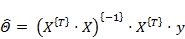
Here,
- The left-hand side of the equation is the value of q that's going to minimize the cost function
- y is a vector containing our target values or labels
Part - 2 - Data generation
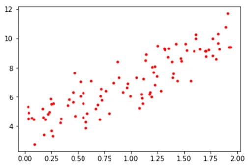
Now, we need data on which we can apply the Normal Equation. Let's create some random data. We need to make sure that the data plot isn't a glorious line, so we're adding some noise to scatter them or create some deviation.
- import numpy as np
- def generate_data():
- X = 2 * np.random.rand(100, 1)
- y = 4 + 3 * X + np.random.randn(100, 1)
- # y = 4 + 3X + Gaussian noise
- # theta_0 or Bias Term = 4
- # theta_1 = 3
- return X, y
Now that our data is created, it is time to fetch our parameters from this dataset. Or we can say getting a value of q that will minimize the cost function.
Part - 3 - Getting
So how do we find the best q? We will use the normal equation.
from numpy.linalg import inv
- def get_best_param(X, y):
- X_transpose = X.T
- best_params = inv(X_transpose.dot(X)).dot(X_transpose).dot(y)
- # normal equation
- # theta_best = (X.T * X)^(-1) * X.T * y
- return best_params # returns a list
Part - 4 - Testing
We have our data, we have 𝛉, so let's test things!
- X, y = generate_data()
- %matplotlib inline
- import matplotlib.pyplot as plt
- plt.plot(X, y, "r.")
- X_b = np.c_[np.ones((100, 1)), X] # set bias term to 1 for each sample
- params = get_best_param(X_b, y)
- print(params)
- array([[ 3.94204397],
- [ 3.08256508]])
Well, the expected values would've been 4 and 3 but we have some noise so deviation is acceptable. [ I'm not saying this is perfect! ]
So how do we get the prediction? Well, another equation,

Here,
- The left-hand side of the equation is the expected output,
- # test prediction
- test_X = np.array([[0], [2]])
- test_X_b = np.c_[np.ones((2, 1)), test_X]
- prediction = test_X_b.dot(params)
- # y = h_Theta_X(Theta) = Theta.T * X
- print(prediction)
- array([[ 3.94204397],
- [ 10.10717414]])
Okay numbers numbers all around. So let's plot the prediction and our dataset in a single graph and see how the model fits the dataset for a regression problem.
- plt.plot(test_X, prediction, "r--")
- plt.plot(X, y, "b.")
- plt.axis([0, 2, 0, 15]) # x axis range 0 to 2, y axis range 0 to 15
- plt.show()
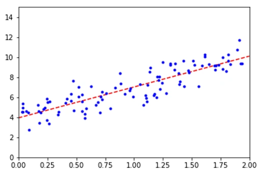
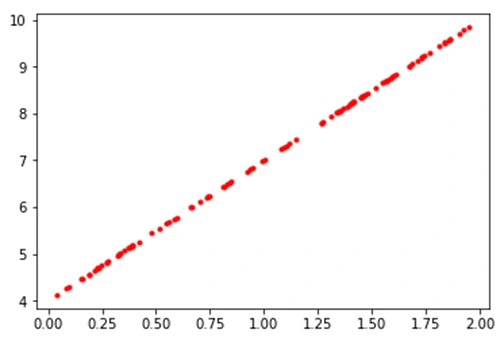
So, we implemented Normal Equation and applied it to predict output for a Linear regression problem. So one curious question - what if we didn't add noise? How would the data plot look? let's find out!
Extra - What if no noise?
- def generate_noiseless_data():
- X = 2 * np.random.rand(100, 1)
- y = 4 + 3 * X
- # y = 4 + 3X
- # theta_0 or Bias Term = 4
- # theta_1 = 3
- return X, y
- X, y = generate_noiseless_data()
- plt.plot(X, y, "r.")
- [<matplotlib.lines.Line2D at 0x10f30f978>]
- X_b = np.c_[np.ones((100, 1)), X] # set bias term to 1 for each sample
- param = get_best_param(X_b, y)
- param
- array([[ 4.],
- [ 3.]])
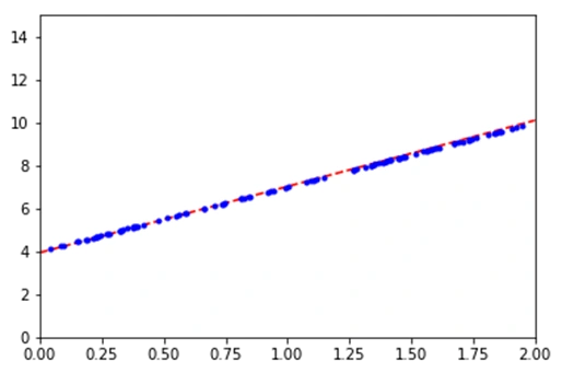
Well well, exactly 4 and 3. For such cases, you don't need machine learning. Just putting values in the line equation does the job.
- test_X = np.array([[0], [2]])
- test_X_b = np.c_[np.ones((2, 1)), test_X]
- prediction = test_X_b.dot(params)
- plt.plot(test_X, prediction, "r--")
- plt.plot(X, y, "b.")
- plt.axis([0, 2, 0, 15]) # x axis range 0 to 2, y axis range 0 to 15
- plt.show()
Join the conversation! Your thoughts help the community grow.