Ultimate End-to-End Guide to TensorFlow: From Installation to Your First Deep Learning Model

Tuhin Paul
1w
256
0
0

Article

TensorFlow is a powerhouse for machine learning and deep learning. It allows us to define the flow of data through multidimensional arrays (tensors) to build complex neural networks. We will cover the exact installation steps for a Windows machine using VS Code, explore the core concepts of Tensors, and finally build a complete Deep Learning project from scratch.

Part 1: Environment Setup & Installation (Windows & VS Code)

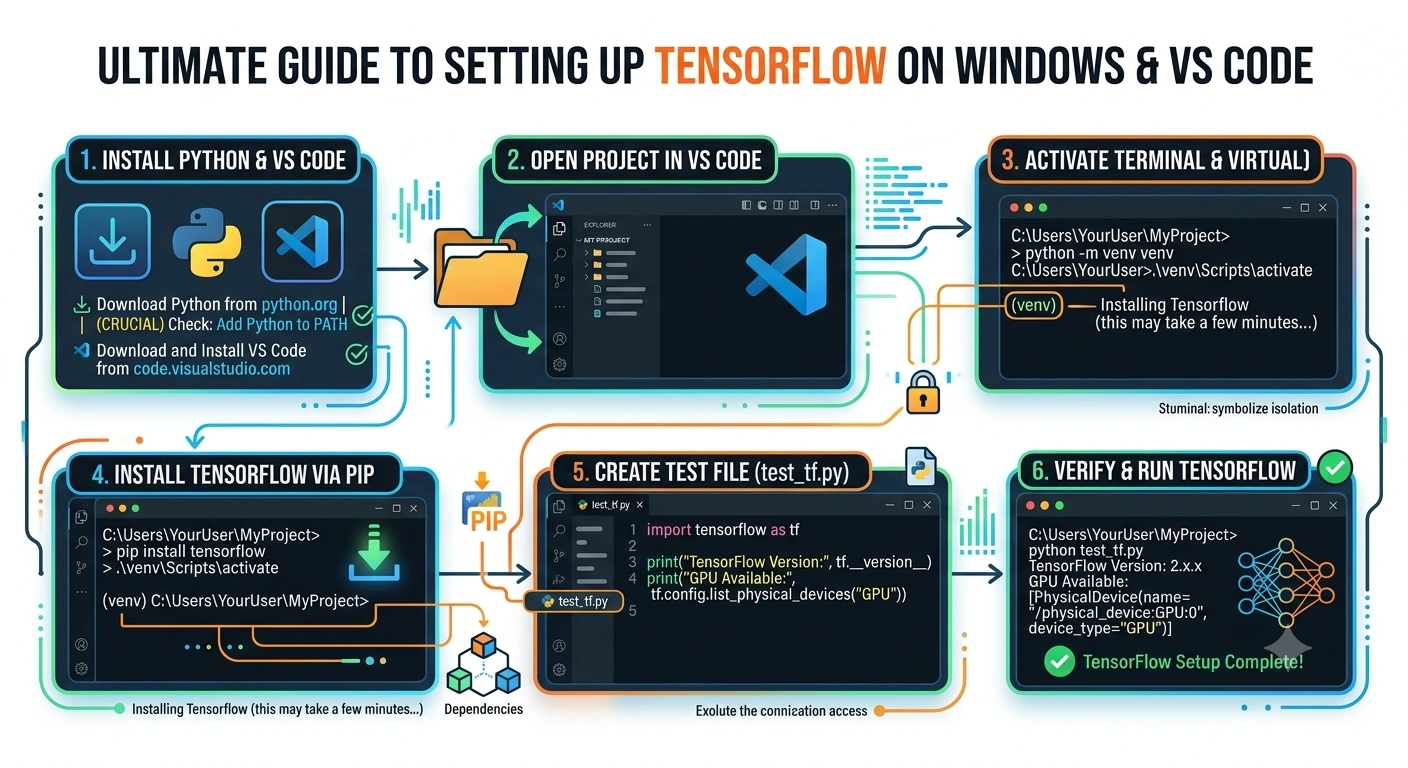
Following the steps you outlined, here is how to set up your TensorFlow environment on a Windows machine.

Step 1 & 2: Install Python and VS Code

Python: Download the latest Python version from python.org. Crucial: During installation, check the box that says "Add Python to PATH".
VS Code: Download and install Visual Studio Code from visualstudio. Install the official Python extension by Microsoft inside VS Code.

Step 3: Setup Virtual Environment (`venv`) in VS Code

A virtual environment keeps your project dependencies isolated.

Open VS Code and open a new folder for your project.
Open the terminal in VS Code (Ctrl + ~ or Terminal > New Terminal).
Create the virtual environment by running:
```
python -m venv venv
```
Activate the virtual environment. In the VS Code terminal (PowerShell or CMD), run:

 .\venv\Scripts\activate

(You will know it worked if you see (venv) at the beginning of your terminal prompt).

Step 4: Install TensorFlow via PIP

With your virtual environment activated, install TensorFlow using pip:

pip install tensorflow

(Note: If you are using an older setup, you might use pip3 install tensorflow, but pip is standard for Python 3.x today).

Step 5 & 6: Testing our TensorFlow

Create a file named test_tf.py and add the following code to verify the installation:

import tensorflow as tf
print("TensorFlow Version:", tf.__version__)
print("GPU Available:", tf.config.list_physical_devices('GPU'))

Run it in the terminal: python test_tf.py. If it prints the version number without errors, you are ready to go!

Part 2: Understanding the Core (Tensors and Flow)

Before building a neural network, let's look at the "Tensor" part of TensorFlow. A tensor is simply a multi-dimensional array.

import tensorflow as tf

# 1. Creating Tensors (Multidimensional arrays)
scalar = tf.constant(7)                     # 0-D Tensor (Scalar)
vector = tf.constant([1, 2, 3])             # 1-D Tensor (Vector)
matrix = tf.constant([[1, 2], [3, 4]])      # 2-D Tensor (Matrix)

# 2. The "Flow" (Operations on Tensors)
# TensorFlow automatically handles the computation flow
tensor_a = tf.constant([[1, 2], [3, 4]])
tensor_b = tf.constant([[5, 6], [7, 8]])

# Addition operation
added_tensors = tf.add(tensor_a, tensor_b)
# Matrix Multiplication operation
multiplied_tensors = tf.matmul(tensor_a, tensor_b)

print("Added:\n", added_tensors)
print("Multiplied:\n", multiplied_tensors)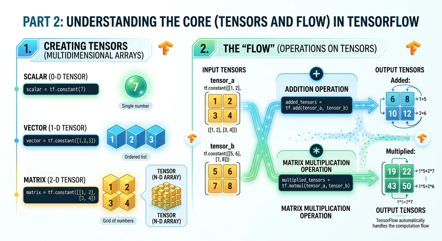

Part 3: End-to-End Deep Learning Project

Now, let's build a complete Deep Learning project. We will create a Neural Network to classify handwritten digits using the famous MNIST dataset.

This project will cover the entire machine learning pipeline:

Loading and Preprocessing Data
Building the Neural Network Architecture
Compiling the Model
Training the Model
Evaluating and Making Predictions

The Complete Code Implementation

Create a new file named mnist_classifier.py and paste the following code. I have added detailed comments to explain the "flow" at every step.

import tensorflow as tf
import matplotlib.pyplot as plt
import numpy as np

print(f"Using TensorFlow Version: {tf.__version__}")

# ==========================================
# 1. LOAD AND PREPROCESS THE DATA
# ==========================================
# TensorFlow/Keras has built-in datasets. We load the MNIST dataset.
mnist = tf.keras.datasets.mnist
(x_train, y_train), (x_test, y_test) = mnist.load_data()

# Preprocessing: Normalize the pixel values to be between 0 and 1.
# This helps the neural network converge faster during training (The "Flow" of data).
x_train, x_test = x_train / 255.0, x_test / 255.0

print(f"Training data shape: {x_train.shape}") # Should be (60000, 28, 28)
print(f"Testing data shape: {x_test.shape}")   # Should be (10000, 28, 28)

# ==========================================
# 2. BUILD THE NEURAL NETWORK MODEL
# ==========================================
# We use the Sequential API, which allows us to build the model layer by layer.
model = tf.keras.models.Sequential([
    # Flatten layer: Converts the 2D array (28x28 image) into a 1D array (784 pixels).
    # No math is done here, it just reshapes the tensor.
    tf.keras.layers.Flatten(input_shape=(28, 28)),
    
    # Dense (Hidden) Layer 1: 128 neurons, ReLU activation function.
    # ReLU (Rectified Linear Unit) introduces non-linearity to the network.
    tf.keras.layers.Dense(128, activation='relu'),
    
    # Dropout Layer: Randomly turns off 20% of neurons during training.
    # This prevents "overfitting" (memorizing the training data).
    tf.keras.layers.Dropout(0.2),
    
    # Output Layer: 10 neurons (one for each digit 0-9). 
    # 'softmax' converts the output into a probability distribution.
    tf.keras.layers.Dense(10, activation='softmax')
])

# ==========================================
# 3. COMPILE THE MODEL
# ==========================================
# We define the optimizer, loss function, and metrics to track.
model.compile(
    optimizer='adam',             # Adam is a highly efficient gradient descent optimizer
    loss='sparse_categorical_crossentropy', # Best for multi-class classification with integer labels
    metrics=['accuracy']          # We want to see accuracy during training
)

# ==========================================
# 4. TRAIN THE MODEL
# ==========================================
# We feed the training data (x_train, y_train) to the model.
# 'epochs' means how many times the model will see the entire dataset.
print("\n--- Starting Training ---")
history = model.fit(x_train, y_train, epochs=5, validation_split=0.1)

# ==========================================
# 5. EVALUATE THE MODEL
# ==========================================
# We test the model on data it has never seen before (x_test, y_test)
print("\n--- Evaluating on Test Data ---")
test_loss, test_acc = model.evaluate(x_test,  y_test, verbose=2)
print(f"\nTest Accuracy: {test_acc*100:.2f}%")

# ==========================================
# 6. MAKE PREDICTIONS
# ==========================================
# Let's use the trained model to predict the first 5 images in the test set.
predictions = model.predict(x_test[:5])

# Display the results
for i in range(5):
    # np.argmax gets the index of the highest probability (the predicted digit)
    predicted_digit = np.argmax(predictions[i])
    actual_digit = y_test[i]
    
    print(f"Image {i+1}: Model Predicts -> {predicted_digit} | Actual Label -> {actual_digit}")
    
    # Optional: Visualize the image using matplotlib
    plt.imshow(x_test[i], cmap=plt.cm.binary)
    plt.title(f"Predicted: {predicted_digit}")
    plt.show()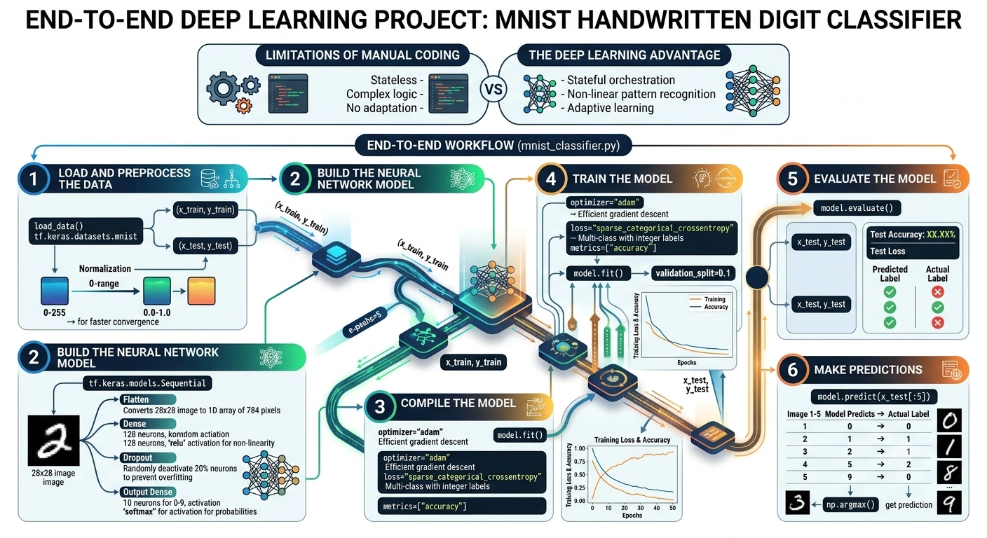

Part 4: Breaking Down the "Flow" in the Code

To tie this back to the core concepts of TensorFlow, here is how the Flow of data happened in our project:

Input Tensors: The images (x_train) entered the network as 2D Tensors of shape (28, 28).
Flatten Operation: The Flatten layer reshaped these 2D Tensors into 1D Tensors of shape (784,) so the dense layers could process them.
Hidden Layer Computations: The Dense layers performed matrix multiplications (tf.matmul) and applied the ReLU activation function to the tensors, extracting features like edges and curves.
Output Tensor: The final Dense layer outputted a 1D Tensor of 10 probabilities (thanks to softmax), representing the model's confidence for each digit from 0 to 9.
Backpropagation (The Learning Flow): During model.fit(), TensorFlow calculated the error (loss) and flowed the gradients backward through the network to update the weights, making the model smarter with every epoch.