


Abstract
Loss functions are central to the development of supervised learning algorithms, particularly neural networks. They provide a quantitative means to evaluate the discrepancy between predicted outputs and actual target values. Beyond their role as optimization objectives, loss functions influence the learning dynamics, convergence behavior, robustness, and generalization capability of a model. This article presents a structured, detailed analysis of loss functions — beginning with the formulation of prediction-level loss, scaling up to empirical loss over datasets, and concluding with an in-depth examination of Binary Cross Entropy and Mean Squared Error, two of the most widely used loss functions in machine learning. The article is then extended to include loss functions for multi-class classification, robust modeling, and reinforcement learning. Real-world examples accompany each concept to contextualize its importance.
1. Quantifying Loss: The Unit of Model Error
The pointwise loss quantifies the error made by a model on a single sample:
𝓛⁽ⁱ⁾ = 𝓛(f(x⁽ⁱ⁾; W), y⁽ⁱ⁾)
Components Breakdown:
- x⁽ⁱ⁾ ∈ ℝᵈ: Input vector.
- y⁽ⁱ⁾: Ground truth label.
- f(x⁽ⁱ⁾; W): Model prediction.
- 𝓛: Chosen loss function.
Scientific Motivation
- Differentiable to support gradient-based optimization.
- Reflects sample-wise performance.
- Not directly minimized, but used to compute stochastic gradients.
Real-Life Example
Medical Diagnosis
If f(x¹) = 0.1 and y¹ = 1, the low probability of illness despite the patient being sick results in a high pointwise loss. This has high impact in medical applications due to the asymmetric cost of false negatives.
2. Empirical Loss: Dataset-Level Performance Metric
Empirical loss aggregates individual losses:
J(W) = (1/n) Σ 𝓛(f(x⁽ⁱ⁾; W), y⁽ⁱ⁾)
Interpretation
- Approximates the true expected risk over distribution 𝓓.
- Key component of Empirical Risk Minimization (ERM).
Regularization
J_reg(W) = J(W) + λ · Ω(W)
To prevent overfitting.
Real-Life Example
A diagnosis model misclassifying certain populations raises overall empirical loss, alerting practitioners to fairness or generalization issues.
3. Binary Cross Entropy (BCE): Loss for Binary Classification
𝓛_BCE = -[y log(ŷ) + (1 - y) log(1 - ŷ)]
Where ŷ = f(x; W) ∈ (0, 1)
Why BCE?
- Derived from Bernoulli likelihood.
- Penalizes confident mispredictions.
Gradient Behavior
Explodes near 0 or 1, encouraging calibrated confidence.
Real-Life Example
Spam Filter
If ŷ = 0.8, y = 0, loss is high ≈ 1.609. The model learns not to be overconfident without evidence.
4. Mean Squared Error (MSE): Canonical Loss for Regression
𝓛_MSE = (y⁽ⁱ⁾ - ŷ⁽ⁱ⁾)²
J(W) = (1/n) Σ (y⁽ⁱ⁾ - f(x⁽ⁱ⁾; W))²
Justification
- MLE under Gaussian noise.
- Penalizes large deviations harshly.
Drawbacks
- Sensitive to outliers.
- May benefit from alternatives like Huber loss.
Real-Life Example
Predicting student grades: true 90, predicted 30 → error = 60 → squared error = 3600.
5. Categorical Cross Entropy (CCE): Loss for Multi-Class Classification
𝓛_CCE = -Σ y_k⁽ⁱ⁾ log ŷ_k⁽ⁱ⁾
Where ŷ = softmax(f(x; W)), y is one-hot.
Why CCE?
- Derived from categorical likelihood.
- Works well with softmax activation.
Real-Life Example
Image Classification
If true digit is 4 but model predicts class 2 with high probability, a large loss is incurred.
6. Robust Loss Functions: Handling Outliers and Label Noise
6.1 Huber Loss:
𝓛_δ^Huber =
½(y - ŷ)² if |y - ŷ| ≤ δ
δ(|y - ŷ| - ½δ) otherwise
- Balances sensitivity and robustness.
6.2 Focal Loss
𝓛_Focal = -αₜ (1 - ŷₜ)^γ log(ŷₜ)
- Reduces contribution from easy negatives.
- Ideal for imbalanced datasets.
Real-Life Example
In tumor detection, focal loss improves learning from rare positives.
7. Loss Functions in Reinforcement Learning (RL)
7.1 Temporal Difference (TD) Loss
𝓛_TD = (r + γ maxₐ' Q(s', a'; θ⁻) - Q(s, a; θ))²
- Used in Q-learning to update value estimates.
7.2 Policy Gradient Loss:
𝓛_PG = -E_{π_θ} [ log π_θ(a|s) · A(s, a) ]
- Maximizes expected reward.
Real-Life Example
In autonomous driving, the agent is optimized to take actions (steering, braking) that maximize safety and comfort.
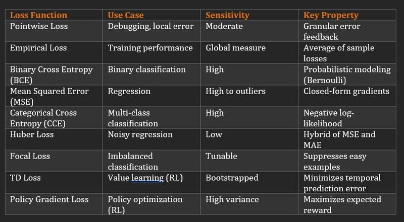
Summary Table: Extended Loss Landscape
Conclusion
Loss functions are more than optimization tools—they define the objectives and behaviors of models, influencing everything from fine-grained prediction accuracy to complex strategies in reinforcement learning. The right choice, informed by scientific rigor and real-world context, is crucial for reliable AI systems.
From the fine-grained view of individual predictions to complex strategies in reinforcement learning, understanding and choosing the appropriate loss function is critical for success in real-world AI systems. Scientific rigor, contextual relevance, and robustness must guide this choice, as the loss landscape shapes how and what a model learns.
Join the conversation! Your thoughts help the community grow.