
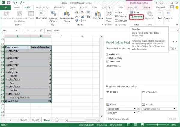
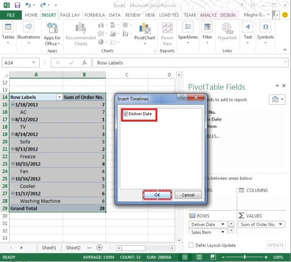
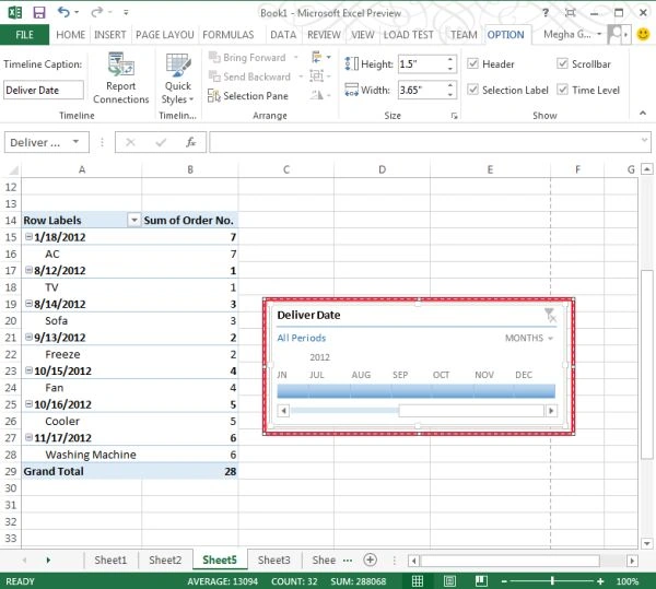
This is a new feature introduced in Excel 2013. This feature is used to filter data that was filled in our sheet. This feature filters the data of the Pivot Table. We can filter the data based on the years, day, month or quarters using the timeline feature. We can filter the Pivot Table data through this new feature of Excel 2013.
Let's have a look at the following steps.
Step 1
Go to Excel 2013.
Step 2
Now select the blank workbook templates from the available templates.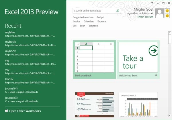
Step 3
Now first fill the sheet with the following data.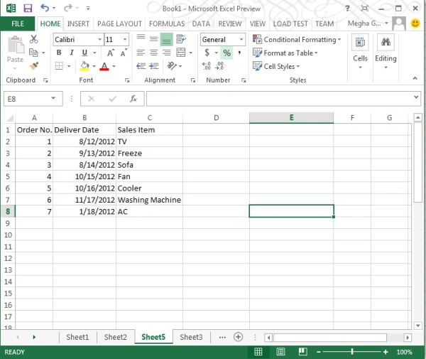
Step 4
Now first we will make a Pivot Table and to do this just select the insert menu option like this: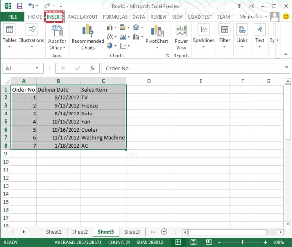
Step 5
And under it just select the Pivot Table option like this: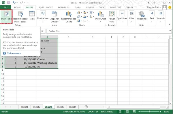
Step 6
Now A create Pivot Table dialog box will appear like this and in it just select the existing Worksheet option like this: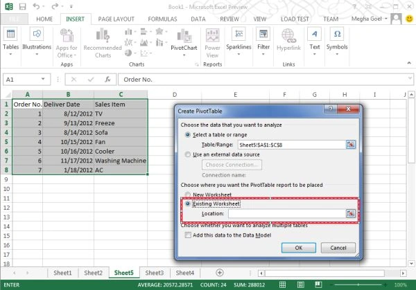
Step 7
Now select some range of the Excel sheet where we want to show the data in the form of a Pivot Table and click on the ok button: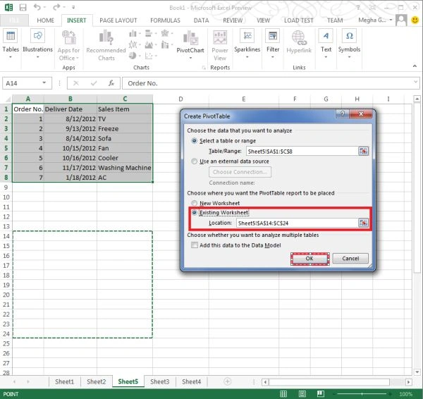
Step 8
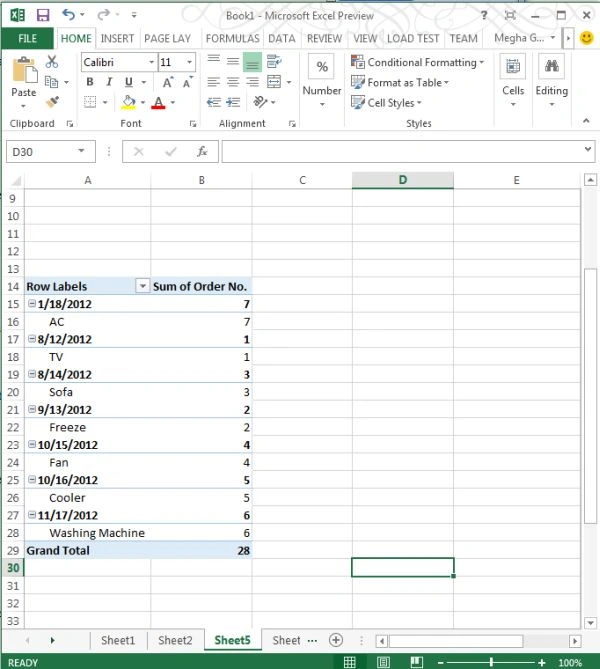
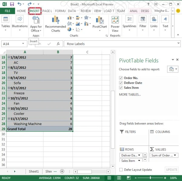
Now select the checkboxes indicating the Pivot Table Fields like this: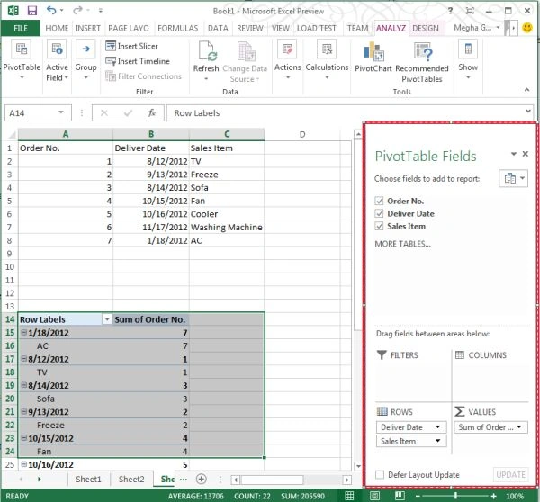
Join the conversation! Your thoughts help the community grow.