Create Report in Power BI Using Power Pivot Tool

This article explains how to import data from SQL Server or any other resource. Really it is very interesting because using any other sources the user imports data using the Power Pivot tool of Power BI.

Now to start with this you need to download Power Pivot in Excel. The following is the link of the Power Pivot for Excel.

What is Power Pivot?

Power Pivot can be used to create discreet and refined data models with Excel data. Power Pivot creates the relationship and custom types of measures between data model. Power Pivot provides better performance by using millions of rows of data. It provides run in memory data model so that business users can analyze the big data very easily. It also works with SQL Server.

These types of tools are not installed previously in Excel, Business users need to download it. The following is the download link for Power Pivot.

Microsoft® SQL Server® 2012 SP1 PowerPivot for Microsoft Excel® 2010

Now start with this procedure.

Step 1: Open Excel sheet

The first and major step is to open an Excel sheet.



Step 2: Select Power Pivot

The second step is to select the Power Pivot tool of Power BI from the menu bar.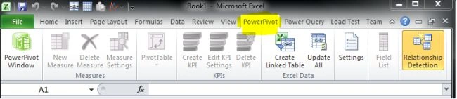



Step 3: Select Power Pivot window

Now the next step is to select the Power Pivot window for importing data.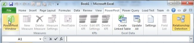



Then this window will be opened.



Step 4: Select from database option

The next step is to select the from database option in the Power Pivot window for importing data from SQL Server.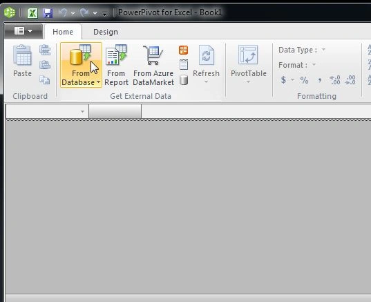



When you select the database option then it shows a list of various options of the database. There are the following three database options.

• From SQL Server
• From Access
• From Analysis Services or Power Pivot

In this article I select the SQL Server database option for importing data in the Power Pivot window.

Step 5: Review the results

After selecting the option from SQL Server, this window will be opened.

Now here the user enters the information required to connect to the SQL Server database.

When the user has entered the information and clicked on the test connection button, then this confirm box will be shown; click on the OK button.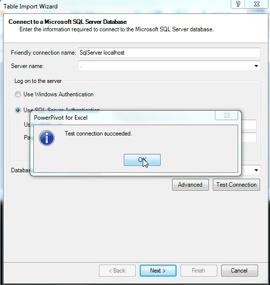



Step 6: Select database name

After checking the test connection, the next step is to select the database name and click on the Next button.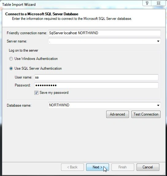



Step 7: Importihng data

It totally depends on the user's choice. In the next step the user needs to select how to import data, either importing all the data from the database table or by writing a query using SQL and then click on the Next button.



Step 8: Select tables from database

The next step is to select the table and views from the database that the user wants to inset as a table in the Power Pivot windows and click on the Finish button.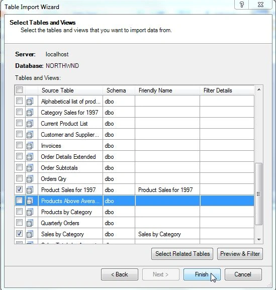



Step 9: Import operation

The import operation takes several minutes to complete. Then the user has seen that the table rows are successfully installed. Then click on the Close button.



Then the user can see the table data.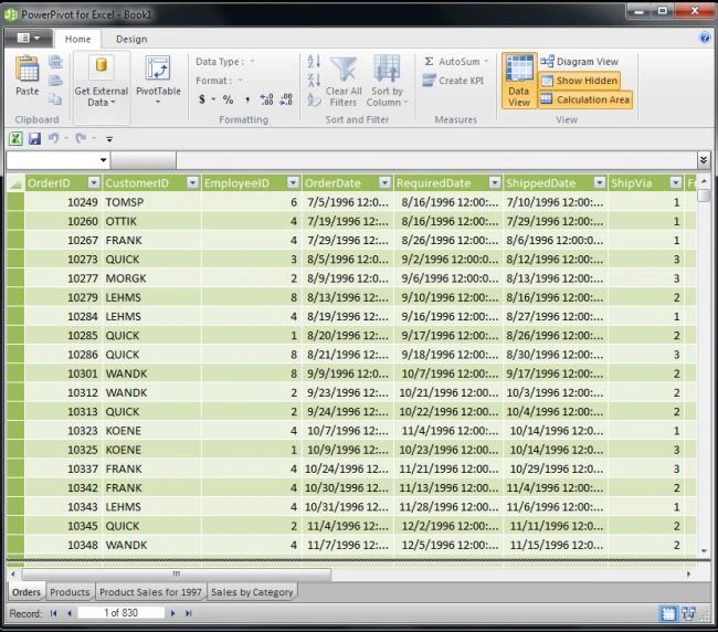



Step 10: Diagram View

If the user wants to see this table data in diagram view then select the diagram view option.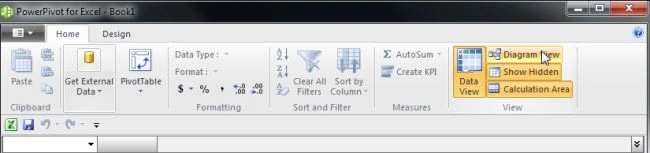



After selecting the diagram view option then the table data will be shown in the diagram view.



Step 11: Select design option

If the user wants to create a relationship between a table and a column then select the design option.

When the user selects the design option, then there is an option for create relationship; select this option to create a relationship.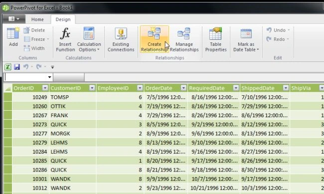



Step 12: Select table and columns

Then the user needs to select a table and columns for creating the relationship and click on the Create button.



The user can create a relationship depending on their choice. Here you can see I create this relationship between tables and columns.



Step 13: Create charts for Power Pivot report

The next step is to select the charts for the report. When the user selects the "pivot table" option then types of chart.

Now here I select the type of the chart.



After selecting the chart option the Excel sheet shows a confirmation box. This confirmation box shows that you want to create a chart in the new Excel sheet or an existing sheet. Then you need to select one option and click on the OK button.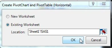



Then this window will be opened. It shows a chart and a table.



Step 14: Drag and drop Power Pivot fields

The next step is to drag and drop Power Pivot fields for the chart and table that we want to show.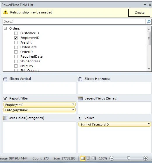



Step 15: Select fields for table

Now here you can see I selected two fields for the Power Pivot table.



Here I created a report depending on my tables and columns.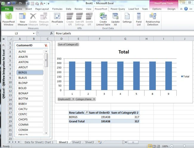



Step 16: Selected data

If I select a row from CustomerID from the table Customer then the Power Pivot charts shows CateogryName and ShipName and Power Pivot tables shows the total number of OrderID and CategoryID. Now you can see this final report.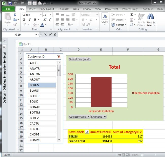



If we select all, rows from CustomerID then it will be shown.



Summary

This article described how to create a Power BI report in Excel using the Power Pivot tool of Power Business Intelligence.

I hope you enjoyed this article.