|
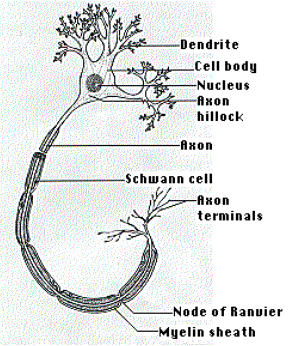
Figure 1(a) - Neuron in the human body
|
|
|
|
|
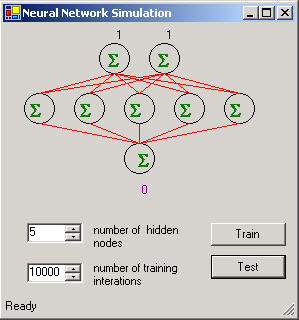
Figure 1(b) - Neural Network XOR Simulation in .Net
Introduction
Although computers are digital systems working on 1's and 0's, our minds function a bit differently. As scientists have explored the working of the human brains, they found that they consist of a network of neurons that communicate with each other through electrical and chemical signals to form our thoughts. These neurons will fire based on the strength and weaknesses of these signals passed between them. The signals are not 1's and 0's, but analog levels with a wide range of potential. As we learn, the neurons in our brain will adjust the potential between these connections, and will develop thresholds and paths that will enforce the associations we receive as input through our senses. Hence, in a way, our brains are more-or-less a 3 pound organic parallel-processing adaptive analog computer.
By simulating a neural network on the computer we can capture one of the greatest capabilities of our brain, the ability to recognize patterns. Neural networks today are used primarily for pattern recognition in applications such as handwriting recognition, stock prediction, and biometric analysis.
In this article we will explore a well-known AI algorithm for modeling the training of neural networks called back propagation. We will use this algorithm to train a neural network to perform an XOR (exclusive or) on its two inputs and to train a prime number detector on its ten inputs.
Neural Network Algorithm
A neural network is simulated on a computer by creating weighted nodes that are interconnected to each other through different layers: the input layer, some hidden layers, and an output layer. A signal passed to an input node in the input layer is multiplied by weights in all the connections to the nodes in the next layer and summed to form an activation value. This value is passed through what is known as a delta function which alters the weighted sum to a non-linear value somewhat simulating how a neuron in the brain would shape the signal. The new activation value is passed on to the next layer and again adjusted by the sum of the weighted values. This process continues until the adjusted value reaches the output layer where it is read.
Training the Network.
In back-propagation, a neural network is trained by comparing the final value occurring at the output of the network to the desired output value and feeding the error backwards through the network and using this error to adjust the weights on the neural nodes. If you send the error back up through the nodes for many iterations, hopefully the weights will eventually converge to values that will make the desired output match the actual output of the network. There is always the possibility that the weights may not converge, or the weights converge to some local minimum that does not provide an optimal solution. By adjusting some of the parameters of the network (number of hidden layers, threshold parameters, number of hidden nodes), you can improve the accuracy of your network.
Once a neural network is trained, you may not ever need to train it again. You can just utilize the final determined weights for all your data. If, however, the input data in your environment is constantly changing (such as in stock predictions), you'll probably find that periodically, you may need to retrain the neural network. Another thing to note about training, is that the output is only as good as the input you give the network. You should use data that statistically covers the broad range of possibilities you expect as input into the network. Also, (as I probably don't need to mention), the desired output must be accurate. As they say in the software industry: "Garbage IN = Garbage OUT".
Back Propogation
One of the best explanations for the back propagation algorithm I found on the web is in an article written by Christos Stergiou and Dimitrios Siganos titled Neural Networks. I'll briefly describe the mathematics and steps of the algorithm here. The first step is the forward pass used to determine the activation levels of the neurons. The forward pass is the same pass used to run the neural net after it is trained. In our example we have only three layers input, hidden, and output. First we will calculate the activation levels of the hidden layer. This is accomplished by input values by the weight matrix between the input layer and the hidden layer and then running the results through a sigmoid function:
1. Lhidden = sigmoid ( Linput * [Weightsinput-hidden])
The sigmoid function is shown below which approaches 1 for large values of x and 0 for very small values of x. This maps all activations to a non-linear approximation of the neuron firing
sigmoid(x)= |
|
The next step in the forward activation is to compute the output layer activations from the hidden layer (in step 1) and the synaptic weight matrix that bridges the hidden layer to the output layer. Then we finally applying the sigmoid to the resulting product matrix.
2. Loutput = sigmoid ( Lhidden * [Weightshidden-output])
That's all there is to the forward pass. Loutput (or the output layer values) contain the results from feeding our initial input into the neural network.
Backward Pass
Once we've calculated the activations for our neurons, we need to calculate the resulting error between the actual output and the desired output. This error is fed back through the neural net and used to adjust the weights to adapt to a more accurate model of our data. The first step is to compute the output layer error:
3. Eoutput = Loutput * (1- Loutput ) * (Loutput - Ldesired)
Now we feed this error into the hidden layer to compute the hidden layer error:
4. Ehidden = Lhidden * (1 - Lhidden ) * [Weightshidden-output ] * Eoutput
Next we need to adjust the weight matrix between the the hidden layer and the output layer to adapt our network and compensate for the error. In order to adjust the weights we'll add two constant factors to our algorithm. The first factor is a learning rate (LR), which adjusts how much the computed error affects the weight change in a single a cycle through the neural net. The second factor is a momentum factor (MF) used in conjunction with the previous weight change to affect the final change in the current cycle through the net. Momentum can often help a network to train a bit faster.
5. [Weightshidden-output ] = [Weightshidden-output ] + D[Weightshidden-output ]
where D[Weightshidden-output ] = (LR) * Lhidden * Eoutput + (MF) * D[Weightshidden-output (previous)]
Finally we need to adjust the weights for the input layer in the same way:
6. [Weightsinput-hidden] =[Weightsinput-hidden] + D[Weightsinput-hidden]
where D[Weightsinput-hidden] = (LR) * Linput * Ehidden + (MF) * D[Weightsinput-hidden(previous)]
After the weights are adjusted, steps 1 through 6 are repeated for the next set of input and desired output values. Once the entire set of data is gone through, we repeat the algorithm for all the data again. This process continues until the network converges or until we choose to stop iterating through the data.
Coding the Back-Propagation Steps:
The code used to implement the back propagation steps is a free download written by Yosif Mohammed. I have just altered the code slightly to allow for repeated training and made it a bit easier to pass training data to the library. Below is the UML diagram describing the neural network reverse engineered using WithClass. The neural network consists of two classes Nnetwork and node. A node contains the weights matrix of the neuron as well as the activation value. The Nnetwork (Neural Network) runs all of the steps of the back propagation using the array of nodes contained in each layer (input, hidden, and output) as seen from the aggregate relationships in the UML diagram.
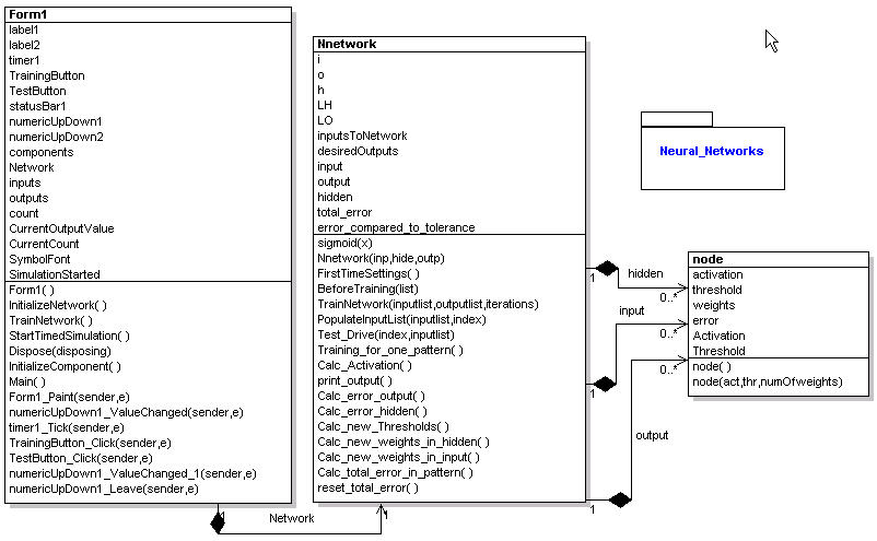
Figure 2 - Neural Network Simulation reverse engineered using WithClass
Steps to running the simulation
When the user presses the Train button in figure 1, the neural network is constructed and the TrainNetwork method of the neural network object is called.
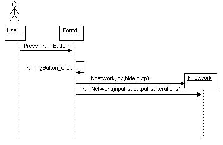
Figure 3 - Training the neural network shown in a UML Sequence diagram in WithClass
The TrainNetwork method repeatedly calls the method Training_for_one_pattern each time for all input and corresponding desired output data sets for n iterations. The value of iterations is passed into the TrainNetwork function from the form, so this value is controlled by the user. Listing 1 contains the code of the TrainNetwork method:
Listing 1 - Training the network with the data from the Form1 object
///
<summary>
/// This function passes training data to the network , inputs and desired ouptus
/// </summary>
/// <param name="list"></param>
public void TrainNetwork(double[,] inputlist, double[,] outputlist, int iterations)
{
// create new arrays to contain input values and desired output values
inputsToNetwork = new double[this.i];
desiredOutputs = new double[this.o];
int outputlistSampleLength = outputlist.GetUpperBound(0) + 1;
int outputlistLength = outputlist.GetUpperBound(1) + 1;
int inputlistLength = inputlist.GetUpperBound(1) + 1;
// copy input and desired output information passed in from the form
for (int i = 0; i < iterations; i++)
{
for (int sampleindex = 0; sampleindex < outputlistSampleLength; sampleindex++)
{
for (int j = 0; j < inputlistLength; j++)
{
inputsToNetwork[j] = inputlist[sampleindex, j];
}
for (int k = 0; k < outputlistLength; k++)
{
desiredOutputs[k] = outputlist[sampleindex, k];
}
// train for the next set of sample input and outputs
Training_for_one_pattern();
}
}
}
The Training_for_one_pattern calls all of the methods that implement steps 1-6 of our back propogation algorithm. Listing 2 is the Training_for_one_pattern method implementing each step.
Listing 2 - Implementing the Back Propagation Algorithm steps 1 - 6
public
void Training_for_one_pattern()
{
// Calculate the Activations for all layers (forward pass steps 1 and 2)
Calc_Activation();
// Calculate the error in the output layer (step 3)
Calc_error_output();
// Calculate the error in the hidden layer (step 4)
Calc_error_hidden();
// Calculate new weights in the hidden layer adjusted with the output layer error (step 5)
Calc_new_weights_in_hidden();
// Calculate new weights in the input layer adjusted with the hidden layer error (step 6)
Calc_new_weights_in_input();
}
Running the Network
Remember that the first steps of the back propagationn algorithm(the forward pass) is the same steps we use to run our neural network after it is trained. The Calc_Activation method of our Neural Network class implements the forward pass shown in Listing 3. In the first part of the method, each node of the input layer is multiplied by the weights between the input and hidden layer and a sigmoid is applied to obtain the form the activation value of the hidden node. In the second part, each node of the hidden layer is multiplied by the weights between the hidden and output layer and a sigmoid is applied to obtain the form the activation value of the output node.
Listing 3 - Forward Pass of the Neural Network (Steps 1 and 2)
///
<summary>
/// a function to calculate the activation of the hidden layer and the output layer
/// </summary>
private void Calc_Activation()
{
// a loop to set the activations of the hidden layer
int ch=0;
while(ch<this.h)
{
for(int ci=0 ; ci<this.i ; ci++)
hidden[ch].Activation += inputsToNetwork[ci] * input[ci].weights[ch];
ch++;
}// end of the while
// calculate the output of the hidden layer
for(int x=0 ; x<this.h ; x++)
{
hidden[x].Activation = sigmoid(hidden[x].Activation );
}
// a loop to set the activations of the output layer
int co=0;
while(co<this.o)
{
for(int chi=0 ; chi<this.h ; chi++)
output[co].Activation += hidden[chi].Activation * hidden[chi].weights[co];
co++;
}// end of the while
// calculate the output of the output layer
for(int x=0 ; x<this.o ; x++)
{
output[x].Activation = sigmoid(output[x].Activation );
}
}
The Neural network utilizes the System.Math library to implement the sigmoid function shown in Listing 4. This function has the signature curve shown adjacent to the code in figure 4. The sigmoid curve causes the values out of a node to act like a neuron. For larger values of input into the neuron, the neuron becomes saturated and reaches a value limit. For smaller values of neuron input, the neuron is less sensitive and tends to stay at a value near zero. For values of input from -0.5 to 0.5, the curve appears to be almost linear giving a proportional mapping of neuron input to output values in this range.
Listing 4 - Sigmoid function
///
<summary>
/// this function to calculate the sigmoid of a double
/// </summary>
/// <param name="x">double number</param>
/// <returns></returns>
private double sigmoid(double x)
{
return 1/(1+Math.Exp(-x));
}
Figure 4 - Sigmoid Curve for different values of x
Training the Neural Net for XOR
Because the neural net is able to handle linear or non-linear mappings, the exclusive or (XOR) is a good simple experiment for testing how well the neural net learns the pattern. The array data below in Listing 5 below is fed into the network to train the weights. The input consists of all the combinations of XOR data for a 2-input system. The outputs represent all of the possible results. Because this is a fairly small closed system, the neural network is not that complex (see Figure 1). The network trains rather quickly after 5000-10000 iterations. With so few nodes, 10000 iterations takes less than a second on a Pentium IV.
Listing 5 - Exclusive OR input and output data
// XOR Data
double[,] inputs = {{0,0}, {0,1}, {1, 0}, {1,1}};
double[,] outputs = {{0}, {1}, {1}, {0}};
Training the Neural Net for Prime Number Recognition
Because this is such a trivial example, I decided to take a look at a little more complex example: training the neural net to recognize prime numbers between 0 and 1000. The data for this example will be entered in binary format. Every prime number from 0-1000 (all 168 of them), are entered into the input as well as all the non-prime numbers from (0-1000). The desired output is "1" if the number is prime and "0" if the number is not prime. The number of input nodes needs to correspond to the number of binary digits in the largest number entered. Since the highest number is 1000, the binary equivalent is around 210 = 1024. Therefore we need 10 input nodes.
Entering binary input data
In order to feed the binary into the network, we constructed a list of all the prime numbers as integers from 1 to 1000 (This was easy enough to find, many web sites have scores of prime number data. Judging from the amount of information out there, I think prime numbers is one of the hottest topics in mathematics). Next we built the prime number binary input and output data dynamically as shown in listing 6:
void
InitializeNetwork()
{
// fill arrays with prime and non prime
for (int i = 0; i < inputs.GetLength(0); i++)
{
// form a binary number from the number i and fill the input array values
int num = i;
int mask = 0x200;
for (int j = 0; j < 10; j++)
{
if ((num & mask) > 0)
inputs[i, j] = 1;
else
inputs[i, j] = 0;
mask = mask >> 1;
}
// check if number appears in the prime number array
// if it does, set the corresponding desired output to 1
// otherwise set the desired output to 0
if (Array.BinarySearch(primes, i) >= 0)
{
// we found a prime
outputs[i,0] = 1;
}
else
{
outputs[i,0] = 0;
}
}
}
Added Features and Network Adjustments
The network seems to work best when the number of hidden nodes in the hidden layer is greater than the number of input nodes. Therefore we chose fifteen input nodes in the hidden layer. The output layer has only one node corresponding to one output determining whether or not we have a prime in the input. Figure 5 shows the Windows Form displaying the rather wide neural network for prime number detection. Note we've added a little bit more functionality to our form including statistics on the trained network and control over the simulation speed. If we want to go through 1000 prime numbers in the simulation, we don't necessarily want the simulation going at one input every 2 seconds, so we give the ability to adjust the amount of time it takes to send each input data set into the network.
Final Results
Figure 5 is a snapshot of the Windows Form after the network already has been trained on 2000 iterations of all numbers from 1-1000. After training, we set the simulation at the highest speed and hit the Test All button. As the simulation flies through 1000 binary numbers, statistics are collected to see if the network contains errors. There are two kinds of errors that can occur in the output: numbers that the network considers prime, but are really composite (non-prime) and numbers that the network considers composite but are really prime. Both statistics are collected at the lower right hand corner of the form. After playing around with the network a bit, I found that increasing the number of nodes in the hidden layer and increasing the number of iterations decreased the error. Of course both adjustments come with the penalty of the amount of time it takes to train the network (a few minutes for 2000 iterations).
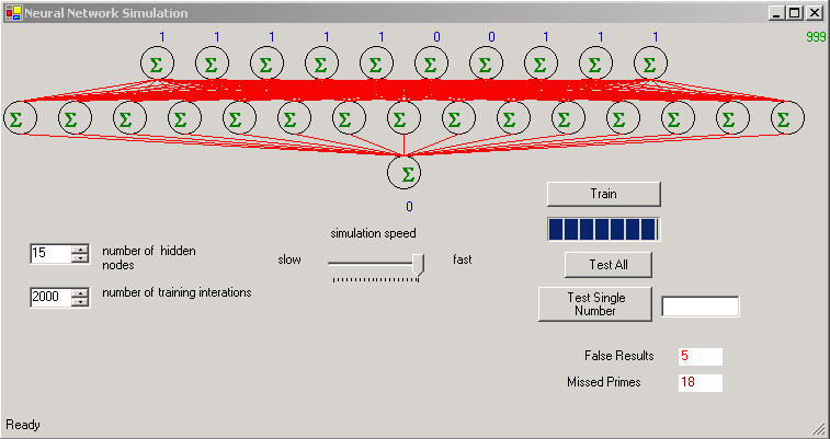
Figure 5 - Prime Number Detector Snapshot after running trained network on 1000 numbers
Conclusion
The neural network, although slow to train, is a powerful way to recognize patterns from known input and output data. For example you can use the network to recognize anything from sounds to handwriting. One cool project you could try would be to create an ink control in the Windows form that allows you to draw characters and then map the characters pixel regions to the input of the neural net. The output could consist of all the possible ascii characters. Another project might be to take a set of sound clips and feed them into the input. Then the output could consist of numbers corresponding to each of the different sound clips. Of course you would need to greatly reduce the number of samples in each clip or somehow just feed certain pertitent samples from the clip, otherwise the number of input nodes would be unwieldy. Anyway have fun running the neural .net and I hope you learned something from this synapsis.