

What is the Simple Linear Regression Model?
Simple Linear Regression is a statistical method that helps to model and analyze the relationship between two continuous variables. In simple linear regression, we have a dependent variable (also known as the response or target variable) and an independent variable (also known as the predictor or explanatory variable).
The relationship between the variables is represented by the equation of a straight line.
- y=mx+b
Where: y is the dependent variable (response), x is the independent variable (predictor), m is the slope of the line (the change in y for a unit change in x), and b is the y-intercept (the value of y when x is 0).
The main goal of simple linear regression is to find the best-fitting line through the data points that minimizes the sum of the squared differences between the observed values (actual data points) and the values predicted by the line. This process is often called "fitting" the model.
The equation of the line is determined during the training phase using a method called the least squares method, which minimizes the sum of the squared vertical distances (residuals) between the observed and predicted values.
Implement Simple Linear Regression in Fabric Notebook
In this article, we are going to use salary data downloaded from kaggle.com. The data is based on the Salary of employees based on experience. The dataset contains two columns, YearsExperience and Salary, respectively.
Step 1. Import the Necessary Python Library
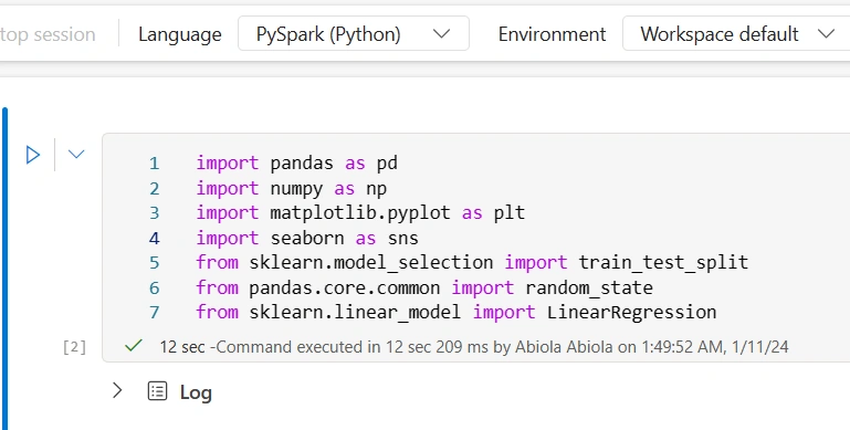
Implementing simple linear regression in Python requires leveraging essential libraries. Pandas is employed for efficient data manipulation, NumPy facilitates mathematical calculations, while Matplotlib and Seaborn handle visualizations. For machine learning operations, Scikit-learn (Sklearn) libraries play a key role. The provided code snippet showcases a basic workflow for building and visualizing a simple linear regression model.
import pandas as pd
import numpy as np
import matplotlib.pyplot as plt
import seaborn as sns
from sklearn.model_selection import train_test_split
from pandas.core.common import random_state
from sklearn.linear_model import LinearRegression
Step 2. Read Data into DataFrame
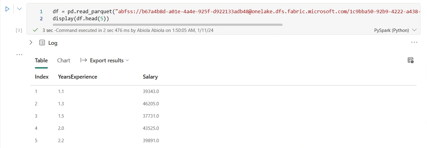
The salary_dataset is initially uploaded into the Simple_Linear_Regression Lakehouse in Microsoft Fabric and then loaded into a Table. To read the parquet file into a DataFrame and display the top 5 records, I executed the code below.
df = pd.read_parquet("abfss://b67a4b8d-a01e-4a4e-925f-d922133adb48@onelake.dfs.fabric.microsoft.com/1c9bba50-92b9-4222-a438-1ed171369403/Tables/salary_data_for_simple_linear_regression_model")
display(df.head(5))
Step 3. Exploratory Data Analysis
Next, I executed the code below to show the dataset descriptive analysis using the describe() method.
df.describe()
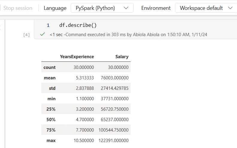
Based on the descriptive analysis, we have 30 records, the smallest salary is 37731, and the highest salary is 122391
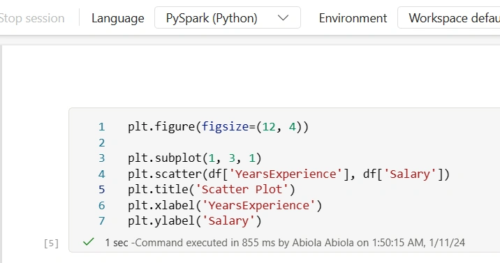
In addition, I explored the relationship between Years of Experience and Salary with a Scatter Plot by firing this code.
plt.figure(figsize=(12, 4))

plt.subplot(1, 3, 1)
plt.scatter(df['YearsExperience'], df['Salary'])
plt.title('Scatter Plot')
plt.xlabel('YearsExperience')
plt.ylabel('Salary')
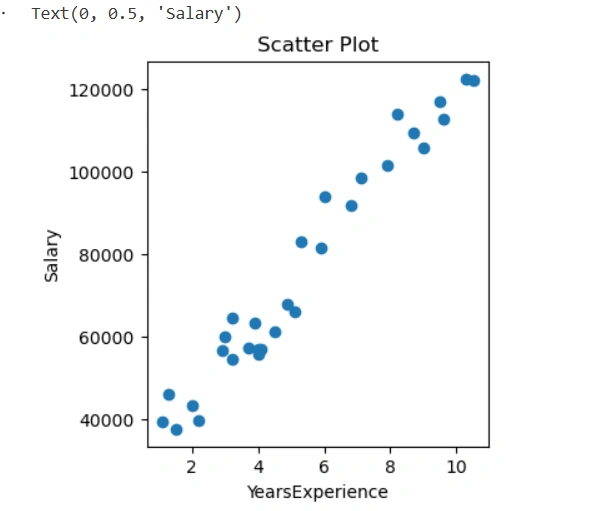
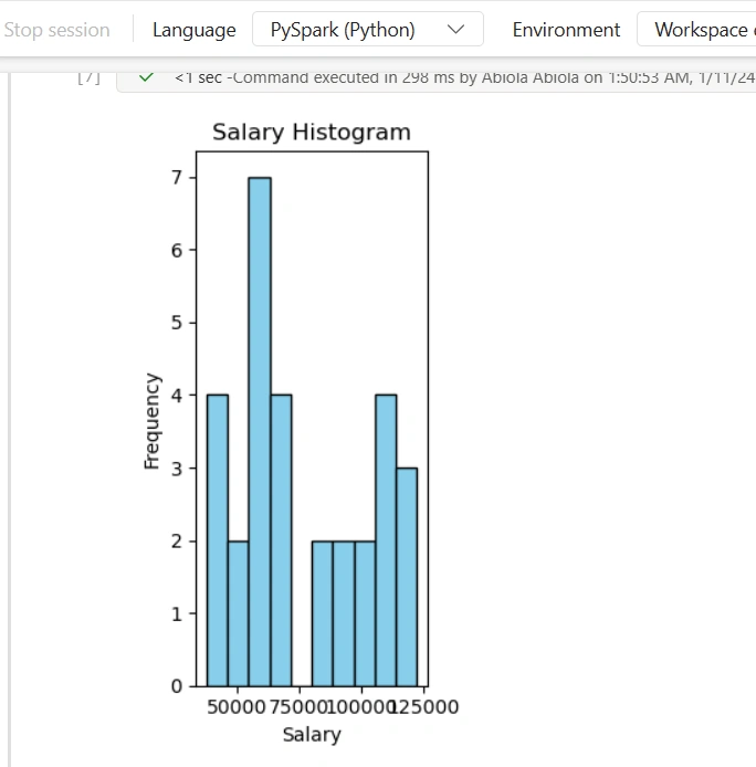
In addition, I also visualize the distribution of Salary using a Histogram by executing this code.
# Histogram
plt.subplot(1, 3, 3)
plt.hist(df['Salary'], bins=10, color='skyblue', edgecolor='black')
plt.title('Salary Histogram')
plt.xlabel('Salary')
plt.ylabel('Frequency')

plt.tight_layout()
plt.show()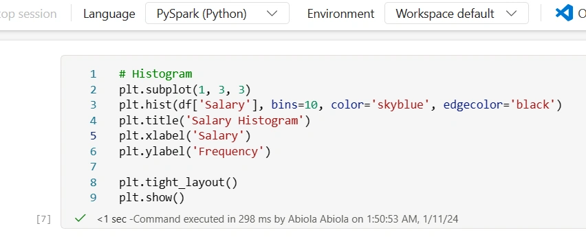
Join the conversation! Your thoughts help the community grow.