Basics of Data Science
Introduction
In the previous chapter, we studied the measure of central tendency in statistics.
In this chapter, we will start with data science, as the name suggests it is the science of data. With of help of which, we can change how data looks, how the data behaviors, or can even exchange data between different formats.
Note: if you can correlate anything with yourself or your life, there are greater chances of understanding the concept. So try to understand everything by relating it to humans.
What is Data?
Data are individual units of information. A datum describes a single quality or quantity of some object or phenomenon. In analytical processes, data are represented by variables. Although the terms "data", "information" and "knowledge" are often used interchangeably, each of these terms has a distinct meaning.
Data is measured, collected and reported, and analyzed, whereupon it can be visualized using graphs, images, or other analysis tools. Data as a general concept refers to the fact that some existing information or knowledge is represented or coded in some form suitable for better usage or processing.
Everything and anything can be called data. Data is an abstract term, which can be used for each and every type of data. The amount of data that is generated on a daily basis can be estimated by seeing the following figures:
- Google: processed 24 Peta Bytes of data every data per day
- Facebook: 10 million photos uploaded every hour
- Youtube: 1 hour of video uploaded every second
- Twitter: 400 million tweets per day
- Astronomy: Satellite Data is in hundreds of petabytes
Note: 1 petabyte is 1 million megabytes or 1 quadrillion bytes or 1000 trillion bytes or 1e^15 bytes
So from the above values, you can very easily understand that on a daily basis we produce around 1 GB or GigaByte of Data. Even the above-written figures are also a type of data.
What is Data Science?
Data Science is a detailed study of the flow of information from the colossal amounts of data present in an organization’s repository. It involves obtaining meaningful insights from raw and unstructured data which is processed through analytical, programming, and business skills.
Data science is a "concept to unify statistics, data analysis, machine learning, and their related methods" in order to "understand and analyze actual phenomena" with data. It employs techniques and theories drawn from many fields within the context of mathematics, statistics, computer science, and information science.
What is Data Munging?
Data wrangling sometimes referred to as data munging, is the process of transforming and mapping data from one "raw" data form into another format with the intent of making it more appropriate and valuable for a variety of downstream purposes such as analytics. A data wrangler is a person who performs these transformation operations.
Raw data can be unstructured and messy, with information coming from disparate data sources, mismatched or missing records, and a slew of other tricky issues. Data munging is a term to describe the data wrangling to bring together data into cohesive views, as well as the janitorial work of cleaning up data so that it is polished and ready for downstream usage. This requires good pattern-recognition sense and clever hacking skills to merge and transform masses of database-level information.
If not properly done, dirty data can obfuscate the 'truth' hidden in the data set and completely mislead results. Thus, any data scientist must be skillful and nimble at data munging in order to have accurate, usable data before applying more sophisticated analytical tactics.
What are the skills required to be a Data Scientist?
A Data Scientist is a professional with the capabilities to gather large amounts of data to analyze and synthesize the information into actionable plans for companies and other organizations. Following are some requirements that need to be met so as to become a good Data Scientist:
1. Mathematic Expertise
At the heart of mining data, insight, and building data products is the ability to view the data through a quantitative lens. There are textures, dimensions, and correlations in data that can be expressed mathematically. Finding solutions utilizing data becomes a brain teaser of heuristics and quantitative technique. Solutions to many business problems involve building analytic models
grounded in hard math, where being able to understand the underlying mechanics of those models is key to success in building them.
2. Technology and Hacking
First, let's clarify that we are not talking about hacking as in breaking into computers. We're referring to the tech programmer subculture meaning of hacking – i.e., creativity and ingenuity in using technical skills to build things and find clever solutions to problems. A data science hacker is a solid algorithmic thinker, having the ability to break down messy problems and recompose them in ways that are solvable.
3. Strong Bussiness Accunme
It is important for a data scientist to be a tactical business consultant. Working so closely with data, data scientists are positioned to learn from data in ways no one else can. That creates the
responsibility to translate observations to shared knowledge and
contribute to strategy on how to solve core business problems
In short, the skills required to be a data scientist are:
- Statistics
- Programming skills
- Critical thinking
- Knowledge of AI, ML, and Deep Learning
- Comfort with math
- Good Knowledge of Python, R, SAS, and Scala
- Communication
- Data Wrangling
- Data Visualization
- Ability to understand analytical functions
- Experience with SQL
- Ability to work with unstructured data
Data Science Components
1. Data (and Its Various Types)
2. Programming (Python and R)
3. Statistics and Probability
4. Machine Learning
5. Big Data
What is Data Science Process?
Data Science Process is the lifecycle of Data Science. It consists of a chronological set of steps. This process is distributed in 6 subparts as:
1. Data Discovery
It includes ways to discover data from various sources which could be in an unstructured format like videos or images or in a structured format like in text files, or it could be from relational database systems.
2. Data Preparation
It includes converting disparate data into a common format in order to work with it seamlessly. This process involves collecting clean data subsets and inserting suitable defaults, and it can also involve more complex methods like identifying missing values by modeling, and so on.
3. Model Planning
Here, you will determine the methods and techniques to draw the relationships between variables. These relationships will set the base for the algorithms which you will implement in the next phase.
4. Model Building
In this phase, you will develop datasets for training and testing purposes. You will consider whether your existing tools will suffice for running the models or it will need a more robust environment (like fast and parallel processing). You will analyze various learning techniques like classification, association, and clustering to build the model.
5. Optimizing
In this phase, you deliver final reports, briefings, code, and technical documents. In addition, sometimes a pilot project is also implemented in a real-time production environment. This will provide you a clear picture of the performance and other related constraints on a small scale before full deployment.
6. Communicate Results
Data Science Python Implementation
By now you all have gained a lot of theoretical knowledge about the concept. Now let's see how do we implement the concept using python.
Here, I am using titanic data, you can download the titanic.csv from kaggle. I am using Google Colab for this, you can use Jupyter Notebook or any other tool for this.
1. Loading Data to Google Colab
To know about Google Colab please click.
There are three ways of uploading a dataset to Google Colab, the following is the way I think is simple, you guys can search and use the other 2 ways.
I use Google Colab, because of the following reasons:
- as unlike Jupyter Notebook, I need not install any libraries
- being a web application, the processing speed is high ( as we get the advantage of using GPUs and TPUs)
- also, we are able to perform Machine Learning on systems with low RAM and system capabilities (I think the most important of all)
- from google.colab import files
- uploaded = files.upload()
2. Preparing the Notebook (Google Colab)
Here, we will be setting up the enviornment of the notebook/Google Colab. And then we will be importing all the required python libraries.
- from IPython.core.display import HTML
- HTML("""
- <style>
- .output_png {
- display: table-cell;
- text-align: center;
- vertical-align: middle;
- }
- </style>
- """);
- %matplotlib inline
- import warnings
- warnings.filterwarnings('ignore')
- warnings.filterwarnings('ignore', category=DeprecationWarning)
- import pandas as pd
- pd.options.display.max_columns = 100
- from matplotlib import pyplot as plt
- import numpy as np
- import seaborn as sns
- import pylab as plot
- params = {
- 'axes.labelsize': "large",
- 'xtick.labelsize': 'x-large',
- 'legend.fontsize': 20,
- 'figure.dpi': 150,
- 'figure.figsize': [25, 7]
- }
- plot.rcParams.update(params)
We will be using pandas to load the dataset.
- data = pd.read_csv('titanic.csv')
- data.shape
Since I am using a CSV file of 891 rows and 12 columns so I will be getting the output as (891,12)
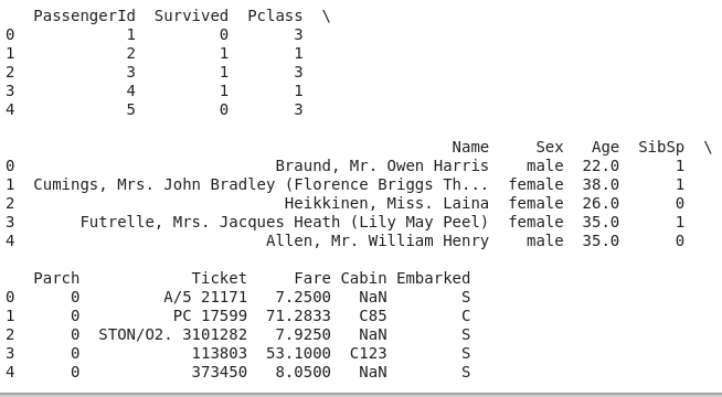
5. Print the top 5 rows of the data
- print(data.head())
6. To get a high-level description of the dataset
- data.describe()
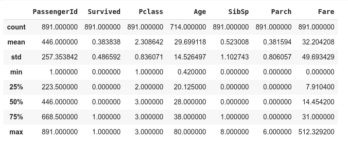
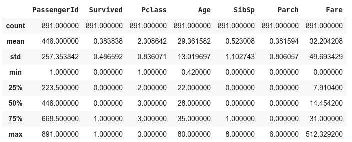
The above output gives us the impression that 177 is missing from the age column, as the count value for age doesnot match with count value of other columns. so to add that we do the following:
- data['Age'] = data['Age'].fillna(data['Age'].median())
7. Data Visualization
Under this topic, we will visualize and try to understand the dataset.
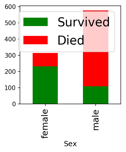
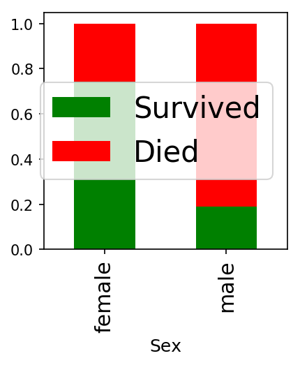
7.1. Visualization of Sex and Survival Chances
- data['Died'] = 1 - data['Survived']
- data.groupby('Sex').agg('sum')[['Survived', 'Died']].plot(kind='bar', figsize=(3, 3),
- stacked=True, colors=['g', 'r']);
We can visualize the above figure in terms of ratios as:
- data.groupby('Sex').agg('mean')[['Survived', 'Died']].plot(kind='bar', figsize=(3, 3),
- stacked=True, colors=['g', 'r']);
7.2. Visualization of the correlation of age variable with men and women
- fig = plt.figure(figsize=(3, 3))
- sns.violinplot(x='Sex', y='Age',
- hue='Survived', data=data, split=True,
- palette={0: "r", 1: "g"});
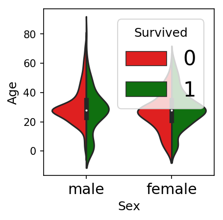
So, from the above, we inferred that women survived more than men
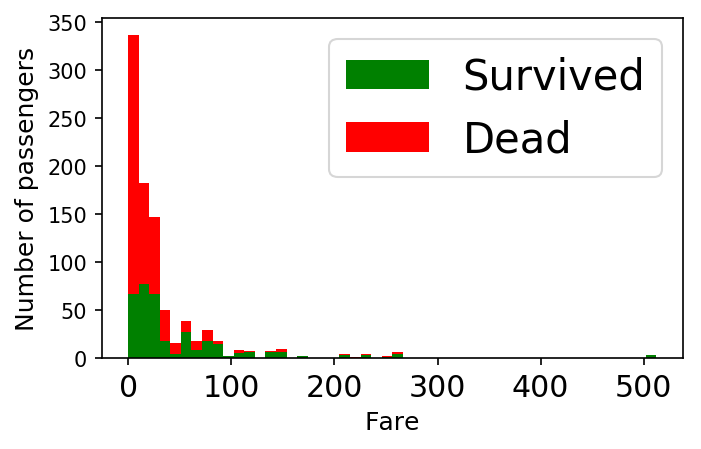
7.3. Visualization of the relationship between fare ticket and their survival chances
- figure = plt.figure(figsize=(5, 3))
- plt.hist([data[data['Survived'] == 1]['Fare'], data[data['Survived'] == 0]['Fare']],
- stacked=True, color = ['g','r'],
- bins = 50, label = ['Survived','Dead'])
- plt.xlabel('Fare')
- plt.ylabel('Number of passengers')
- plt.legend();
7.4. Visualization of the relationship between fare ticket, age, and their survival chances
- plt.figure(figsize=(25, 7))
- ax = plt.subplot()
- ax.scatter(data[data['Survived'] == 1]['Age'], data[data['Survived'] == 1]['Fare'],
- c='green', s=data[data['Survived'] == 1]['Fare'])
- ax.scatter(data[data['Survived'] == 0]['Age'], data[data['Survived'] == 0]['Fare'],
- c='red', s=data[data['Survived'] == 0]['Fare']);
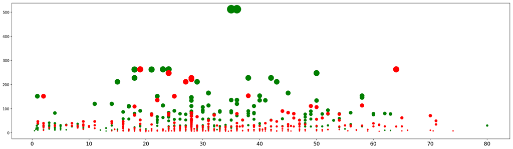
We can observe different clusters:
- Large green dots between x=20 and x=45: adults with the largest ticket fares
- Small red dots between x=10 and x=45, adults from lower classes on the boat
- Small greed dots between x=0 and x=7: these are the children that were saved
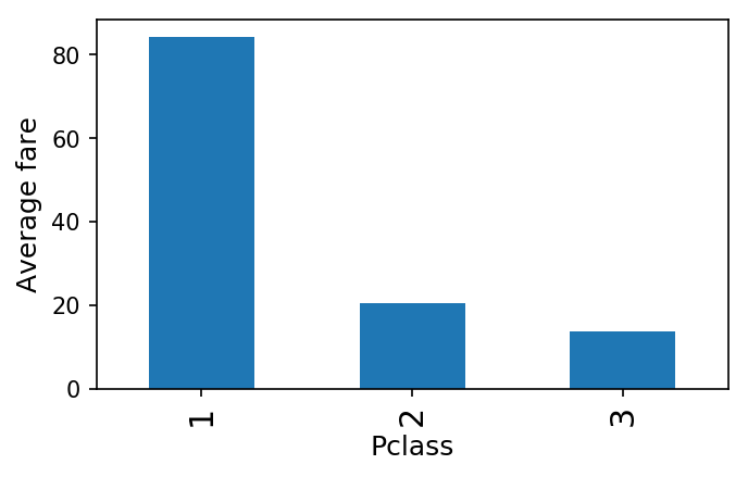
- ax = plt.subplot()
- ax.set_ylabel('Average fare')
- data.groupby('Pclass').mean()['Fare'].plot(kind='bar', figsize=(5, 3), ax = ax);
7.6. Visualization of the relationship between fare ticket, embarked, and their survival chances
- fig = plt.figure(figsize=(5, 3))
- sns.violinplot(x='Embarked', y='Fare', hue='Survived', data=data, split=True, palette={0: "r", 1: "g"});
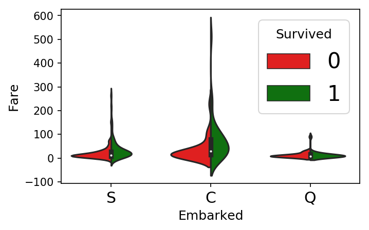
From the above visualization, we can infer that the passengers who paid the highest or who were set in C, survived the most
Data Wrangling Python Implementation
Here we will be cleaning the data so as to make it ready for a machine-learning algorithm to work on it, i.e. will fill missing values, see if the data is continuous or not and see if data need any modifications to be done?
- data.describe()
From the above data, we get the impression that the minimum age of the passengers is 0.42 i.e. 5 months. This is very suspicious as according to the news, we had a two-month-old baby on board, i.e. the minimum age should be 0.19.
Also in the "fare" field, we find some of the values to be (0,0). which either means that those passengers traveled free or the data is missing.
So, let us first check whether any of the cells in the data is empty or not?
- data.count()
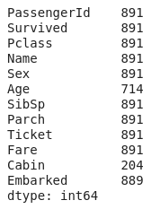
So from the above, output it is crystal clear that we have some data missing or the corresponding cells are empty in the "embarked", "age" and "cabin" columns.
So, what to do now. Either we have to delete the columns with missing data or we did have to fill the missing places. Now, I will be telling you how I reduce the number of missing values.
There are three ways to fill the missing value
1. Replace each cell with value '0' with numpy.NaN
- data = data.replace(0, np.NaN)
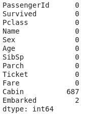
- print(data.isnull().sum())
So, we can see that to some extent we were able to clean the data, but some of the data got corrupted. So let's try another way and see the result
2. Replace each missing value by the Column Mean
- data.fillna(data.mean(), inplace=True)
- # count the number of NaN values in each column
- print(data.isnull().sum())
Here, we see that we were able to rectify "age" and also nothing got corrupted. But we were not able to rectify "cabin" and "embarked". So now let's try another way.
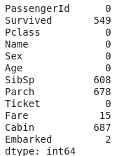
3. Replacing each numpy.NaN value with zero
- data = data.replace(np.NaN, 0)
- # count the number of NaN values in each column
- print(data.isnull().sum())
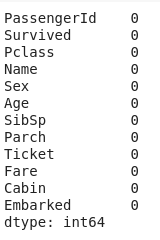
So, by using this I was able to achieve a "no null" situation.
Note: But replacing missing values I had achieved but it is quite possible that it may result in loss of data or may change the meaning of data.
Conclusion
In this chapter, we studied data science.
In the next chapter, we will learn about machine learning and some commonly used terms with it.
Author

Rohit Gupta
13
60.9k
3.2m