Machine Learning Project 2: IRIS dataset
Introduction
This chapter demonstrates a machine learning application using the IRIS dataset.
IRIS Dataset
Iris data set is the famous smaller databases for easier visualization and analysis techniques.
1. Environment setup
- Download and install Anaconda navigator, which is distributed a variety of integrated development environments for scientific programming and data analyst as without using any command-line commands.
- The spyder IDE provides better interactive editing and debugging facilities for data analysis.
- To check out necessary libraries that have been installed or not with their versions.
-
- import pandas
- print('pandas version is: {}'.format(pandas.__version__))
- import numpy
- print('numpy version is:{}'.format(numpy.__version__))
- import seaborn
- print('seaborn version is{}'.format(seaborn.__version__))
- import sklearn
- print('sklearn version is:{}'.format(sklearn.__version__))

2. Load and understanding data
 2.2 Understanding the dataset
Here, we are going to do a few tasks to understand how numerical data has categorized.
- Pandas is a python package that provides fast and flexible data analysis to the relational or labeled database.
- Before loading the dataset, you should store the dataset in the spyder working directory.
2.1 Loading the dataset
- #load dataset
- import pandas as PD
- iris=pd.read_csv('Iris.csv')

2.2.1 Preview data
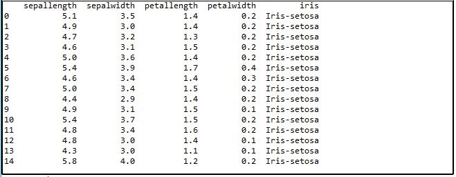
Let’s, look at the iris flowers numerical data belongs to their four species. You can see a first 15 numerical row of species. If the dataset contains three types of flower sets called Iris virginica, Versicolor, and iris Sentosa. These three flower features are measured along with their species.
- #preview data
- print(iris.head(15))
2.2.2 Description of dataset
Let’s look at a summary of each iris instance attributes.
- #Description of Data
- print(iris.describe())
If the four features of iris species measured by count, min, mean, max, and percentiles.

2.2.3 Description of class
Now, the time to view how many instances the data frame contains.
- #Flower distribution
- print(iris.groupby('iris').size())
If the dataset contains three classes with 150 instances and its entire instances were measured as numerical values by their features.

2.2.4 Shape of Data
The shape property provides us to seek entire counts of flower instances.
- #Data Shape
- print(iris.shape)
There is a data frame contains 150 samples under the 5 columns.
3. Data visualization
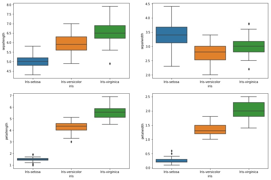
- The visualization techniques provide imagery representation of Iris species and feature It is used to determine correlations between the X and Y variables (dependent and independent variables).
- Now, we are going to visualize the dataset in two ways such as Boxplot, and pairwise joint plot distribution (scatter plot).
3.1 Boxplot
- The graph represented the shape of data distribution and their upper and lower quartiles.
- The iris species might show with few box plot standard ways such as mean, median, and deviation.
-
- #Boxplot
- plt.figure(figsize=(15,10))
- plt.subplot(2,2,1)
- sns.boxplot(x='iris',y='sepallength',data=iris)
- plt.subplot(2,2,2)
- sns.boxplot(x='iris',y='sepalwidth',data=iris)
- plt.subplot(2,2,3)
- sns.boxplot(x='iris',y='petallength',data=iris)
- plt.subplot(2,2,4)
- sns.boxplot(x='iris',y='petalwidth',data=iris)
3.2 Pair plot
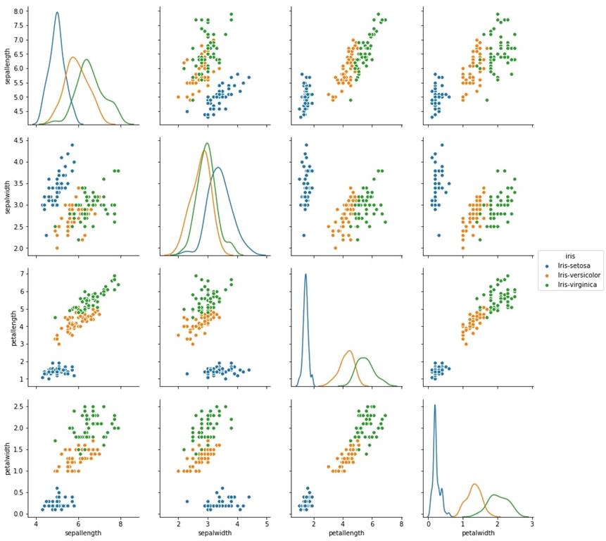
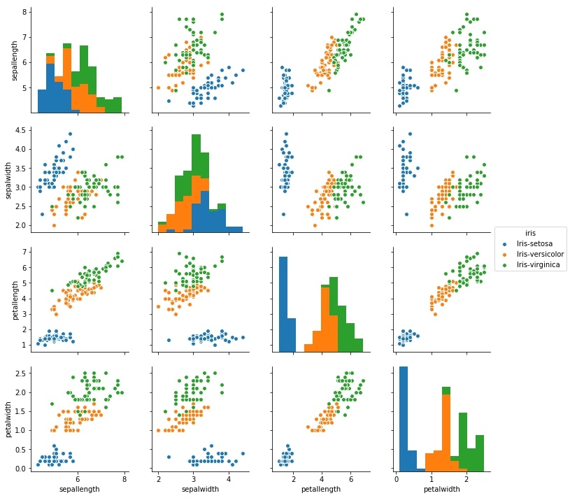
The pair plot used to figure out a distribution of single variables and the relationship between two variables. If the pair plot is given a solution for that as a clear understanding of each flower sets at a single graph. Each flower scatters plots represented in different colors.
- #Pairwise joint plot (scatter matrix)
- sns.pairplot(iris, hue='iris', size=3, diag_kind="kde")
- sns.pairplot(iris,hue='iris')
Here, it also appears some overleaping data points.
4. Train and validate data (Machine learning)
Here, we’ll separate the dataset into two parts for validation processes such as train data and test data. Then allocating 80% of data for training tasks and the remainder 20% for validation purposes.
- #dataset spliting
- array = iris.values
- X = array[:,0:4]
- Y = array[:,4]
- validation_size = 0.20
- seed = 7
- X_train, X_validation, Y_train, Y_validation = cross_validation.train_test_split(X, Y, test_size=validation_size,
- random_state=seed)
- #k=10
- num_folds = 10
- num_instances = len(X_train)
- seed = 7
- scoring = 'accuracy'
4.1 Train the model (Modeling)
- Now, it's time to determine the best suitable algorithm for getting effective accuracy.
- Here, we are going to evaluate five famous frequently used algorithms such as
- Linear regression algorithm
- Logistic regression
- Decision tree classifier
- Gaussian Naïve Base
- Support Vector Machine
- #evaluate model to determine better algorithm
- models = []
- models.append(('LR', LogisticRegression()))
- models.append(('LDA', LinearDiscriminantAnalysis()))
- models.append(('CART', DecisionTreeClassifier()))
- models.append(('NB', GaussianNB()))
- models.append(('SVM', SVM()))
- results = []
- names = []
- for name, model in models:
- kfold = cross_validation.KFold(n=num_instances, n_folds=num_folds, random_state=seed)
- cv_results = cross_validation.cross_val_score(model, X_train, Y_train, cv=kfold, scoring=scoring)
- results.append(cv_results)
- names.append(name)
- msg = "%s: %f (%f)" % (name, cv_results.mean(), cv_results.std())
- print(msg)
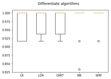
The support vector machine model appears a high score of accuracy.

4.2 Algorithm comparison
You can also discover better accuracy by the algorithm comparison graph.
- #choose best one model trough graphical representation
- plt.figure(figsize=(15,10))
- fig = plt.figure()
- fig.suptitle('Differentiate algorithms')
- ax = fig.add_subplot(111)
- plt.boxplot(results)
- ax.set_xticklabels(names)
- plt.show()
5. Validate the data(prediction)
Let’s predict a value by validation.
- #pretiction
- svn = SVM()
- svn.fit(X_train, Y_train)
- predictions = svn.predict(X_validation)
- print(accuracy_score(Y_validation, predictions))
- print(confusion_matrix(Y_validation, predictions))
- print(classification_report(Y_validation, predictions))

Testing the new data.
- #verify new data
- X_new = numpy.array([[3, 2, 4, 0.2], [ 4.7, 3, 1.3, 0.2 ]])
- print("X_new.shape: {}".format(X_new.shape))
Validating the prediction
- #validate
- prediction = svn.predict(X_new)
- print("Prediction of Species: {}".format(prediction))
Conclusion
So in this chapter, you learned how to build an application using the IRIS dataset.
Author
Elavarasan R
0
11.4k
672.7k
