Machine Learninig: Decision Tree
Introduction
In the previous chapter, you studied Multiple Linear Regression.
In this chapter, we will study Multiple Linear Regression.
Note: if
you can correlate anything with yourself or your life, there are greater chances of understanding the concept. So try to understand everything by relating it to humans.
What is Decision Tree?
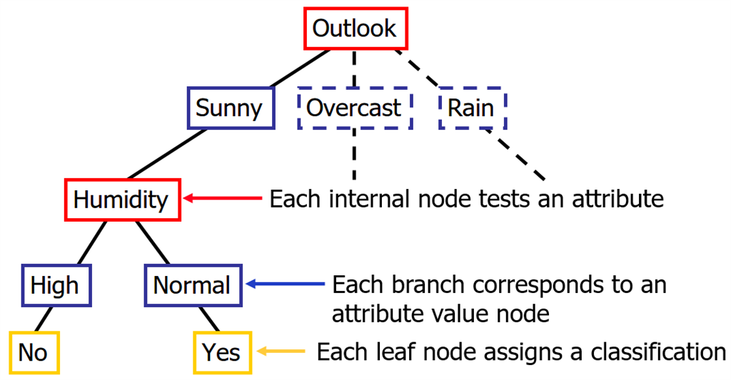
A decision tree is a decision support tool that uses a tree-like graph or model of decisions and their possible consequences, including chance event outcomes, resource costs, and utility. It is one way to display an algorithm that only contains conditional control statements.
Decision Trees (DTs) are a non-parametric supervised learning method used for both classification and regression. Decision trees learn from data to approximate a sine curve with a set of if-then-else decision rules. The deeper the tree, the more complex the decision rules, and the fitter the model.
The decision tree builds classification or regression models in the form of a tree structure, hence called CART (Classification and Regression Trees). It breaks down a data set into smaller and smaller subsets building along an associated decision tree at the same time. The final result is a tree with decision nodes and leaf nodes. A decision node has two or more branches. The leaf node represents a classification or decision. The topmost decision node in a tree which corresponds to the best predictor called the root node. Decision trees can handle both categorical and numerical data.
When is Decision Tree Used?
- When the user has an objective he is trying to achieve: max profit, optimize cost
- When there are several courses of action
- There is a calculated measure of the benefit of the various alternatives
- When there are events beyond the control of the decision-maker i.e environment factor.
- Uncertainty concerning which outcome will actually happen
Assumptions of Decision Tree
- In the beginning, the whole training set is considered as the root.
- Feature values are preferred to be categorical. If the values are continuous then they are discretized prior to building the model.
- Records are distributed recursively on the basis of attribute values.
- Order to placing attributes as root or internal node of the tree is done by using some statistical approach.
Key Terms
- Root Node - It represents the entire population or sample and this further gets divided into two or more homogeneous sets.
- Splitting - It is a process of dividing a node into two or more sub-nodes.
- Decision Node - When a sub-node splits into further sub-nodes, then it is called a decision node.
- Leaf/ Terminal Node - Nodes do not split is called Leaf or Terminal node.
- Pruning - When we remove the sub-nodes of a decision node, this process is called pruning. You can say the opposite process of splitting.
- Branch / Sub-Tree - A subsection of the entire tree is called branch or sub-tree.
- Parent and Child Node - A node, which is divided into sub-nodes is called the parent node of sub-nodes whereas sub-nodes are the child of the parent node.
- Entropy - A decision tree is built top-down from a root node and involves partitioning the data into subsets that contain instances with similar values (homogeneous). ID 3 algorithm uses entropy to calculate the homogeneity of a sample. If the sample is completely homogeneous the entropy is zero and if the sample is equally divided it has an entropy of one.
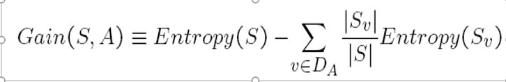
- Information Gain - The information gain is based on the decrease in entropy after a dataset is split on an attribute. Constructing a decision tree is all about finding an attribute that returns the highest information gain (i.e., the most homogeneous branches).
- Internal Node - An internal node (also known as an inner node, inode for short, or branch node) is any node of a tree that has child nodes
- Branch - The lines connecting elements are called "branches".
How to Make a Decision Tree?
Step 1
Calculate the entropy of the target.
Step 2
The dataset is then split into different attributes. The entropy for each branch is calculated. Then it is added proportionally, to get total entropy for the split. The resulting entropy is subtracted from the entropy before the split. The result is the Information Gain or decrease in entropy.
Step 3
Choose attribute with the largest information gain as the decision node, divide the dataset by its branches, and repeat the same process on every branch.
Types of Decision Tree
- Categorical Variable Decision Tree
Decision Tree which has a categorical target variable then it called a categorical variable decision tree. For Example, I say Will Bangladesh be able to beat India?, so I can have the decision parameter as YES or NO. - Continuous Variable Decision Tree
Decision Tree has a continuous target variable then it is called Continuous Variable Decision Tree. For Example, I say What is the percentage of chances that India will win? so here we have a varying value. - ID3 (Iterative Dichotomiser 3)
- C4.5 (successor of ID3)
- CART (Classification And Regression Tree)
- CHAID (CHi-squared Automatic Interaction Detector)
- MARS (Multivariate Adaptive Regression Splines)
- Conditional Inference Trees.
What is the importance of a Decision Tree?
- Simple to easy, use, understand and explain
- They do feature selection and variable screening
- They require very little efforts to prepare and produce
- Can live with nonlinear relationships and parameters also
- Can use conditional probability-based reasoning or Bayes theorem
- They provide strategic answers to uncertain situations
Regression Tree vs Classification Tree
| Regression Tree | Classification Tree | |
| Dependent Variable | Used when the dependent variable is continuous | Used when the dependent variable is categorical |
| Unseen Data | Makes prediction with the mean value | Makes prediction with mode values |
| Predictor Space | divides into a distinct and non-overlapping region | divides into a distinct and non-overlapping region |
| Approach Followed | Top-Down Greedy | Top-Down Greedy |
Entropy and Information Gain Calculations
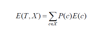
Entropy is something that is very important when we have to find the Information Gain, which in turn places a vital role in selecting the next attribute.
Following is the formula we will use during this article,
Example 1
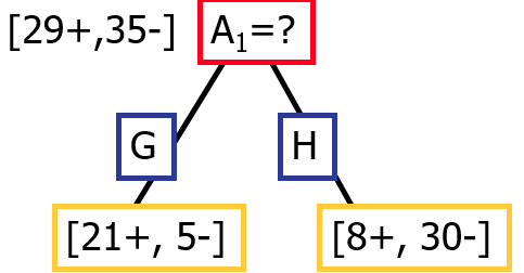
Entropy([29+,35-]) = -29/64*log2 (29/64) – 35/64*log2 (35/64)
= 0.99
Entropy([21+,5-]) = -21/26*log2 (21/26) - 5/26*log2 (5/26)
= 0.71
Entropy([8+,30-]) = -8/38*log2 (8/38) - 30/38 *log2 (30/38)
= 0.74
Information Gain([29+,35-]),A1) = 0.99 - (26/64)*0.71 - (38/64)*0.74
=-0.15
Example 2
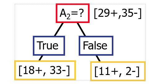
Entropy([29+,35-]) = -29/64*log2 (29/64) – 35/64*log2 (35/64)
= 0.99
Entropy([21+,5-]) = -18/51*log2 (18/51) - 33/51*log2 (33/51)
= 0.94
Entropy([8+,30-]) = -11/13*log2 (11/13) - 2/13 *log2 (2/13)
= 0.62
Information Gain([29+,35-]),A1) = 0.99 - (52/64)*0.94 - (13/64)*0.62
=0.1
So we can see that the information gain is bigger incase of example 2(IG=0.1) as compared to example 1(IG=-0.15)
Decision Tree Example
Till now we studied theory, now let's try out some hands-on. I will take a demo dataset and will construct a decision tree based upon that dataset.
I am taking the following dataset, where we make a decision on whether we will play or not based upon the given environmental conditions.
| Day | Outlook | Temperature | Humidity | Wind | Play Tennis |
| D1 | Sunny | Hot | High | Weak | No |
| D2 | Sunny | Hot | High | Strong | No |
| D3 | Overcast | Hot | High | Weak | Yes |
| D4 | Rain | Mild | High | Weak | Yes |
| D5 | Rain | Cool | Normal | Weak | Yes |
| D6 | Rain | Cool | Normal | Strong | No |
| D7 | Overcast | Cool | Normal | Weak | Yes |
| D8 | Sunny | Mild | High | Weak | No |
| D9 | Sunny | Cool | Normal | Weak | Yes |
| D10 | Rain | Mild | Normal | Strong | Yes |
| D11 | Sunny | Mild | Normal | Strong | Yes |
| D12 | Overcast | Mild | High | Strong | Yes |
| D13 | Overcast | Hot | Normal | Weak | Yes |
| D14 | Rain | Mild | High | Strong | No |
Calculation of Gini Index for "Outlook" feature
1. We can see that Outlook has 5 instances (5/14) as "Sunny", 4 instances (4/14) as "Overcast" and 5 instances as "Rain".
2. Outlook = Sunny, Play Tennis = Yes, we have 2 instances (2/5)
Outlook = Sunny, Play Tennis = No, we have 3 instances (3/5)
Hence, the Gini Index comes out to be:
= 1 - ((2/5)^2+(3/5)^2)
= 0.48
3. Outlook = Overcast, Play Tennis = Yes, we have 4 instances (4/4)
Outlook = Overcast, Play Tennis = No, we have 0 instances (0/4)
Hence, the Gini Index comes out to be:
= 1 - ((4/4)^2+(0/4)^2)
= 0
4. Outlook = Rain, Play Tennis = Yes, we have 3 instances (3/5)
Outlook = Rain, Play Tennis = No, we have 2 instances (2/5)
Hence, the Gini Index comes out to be:
= 1 - ((3/5)^2+(2/5)^2)
= 0.48
5. So the final Gini Index is:
= (5/14)*0.48 + (4/14)*0 + (5/14)*0.48
= 0.34
Calculations of Gini Index of "Temperature" feature
1. We can see that, Temperature has 4 instances (4/14) as "Hot", 4 instances (4/14) as "Cool", 6 instances (6/14) as "Mild"
2. Temperature = Hot, Play Tennis = Yes, we have 2 instances (2/4)
Temperature = Hot, Play Tennis = No, we have 3 instances (2/4)
Hence, the Gini Index comes out to be:
= 1 - ((2/4)^2+(2/4)^2)
= 0.5
3. Temperature = Cool, Play Tennis = Yes, we have 3 instances (3/4)
Temperature = Cool, Play Tennis = No, we have 1 instances (1/4)
Hence, the Gini Index comes out to be:
= 1 - ((3/4)^2+(1/4)^2)
= 0.375
4. Temperature = Mild, Play Tennis = Yes, we have 4 instances (4/6)
Temperature = Mild, Play Tennis = No, we have 2 instances (2/6)
Hence, the Gini Index comes out to be:
= 1 - ((4/6)^2+(2/6)^2)
= 0.44
5. So the final Gini Index is:
= (4/14)*0.5 + (4/14)*0.375 + (6/14)*0.44
= 0.44
Calculations of Gini Index of "Humidity" feature
2. Humidity = High, Play Tennis = Yes, we have 3 instances (3/7)
Humidity = High, Play Tennis = No, we have 4 instances (4/7)
Hence, the Gini Index comes out to be:
= 1 - ((3/7)^2+(4/7)^2)
= 0.49
3. Humidity = Normal, Play Tennis = Yes, we have 6 instances (6/7)
Humidity = Normal, Play Tennis = No, we have 1 instance (1/7)
Hence, the Gini Index comes out to be:
= 1 - ((6/7)^2+(1/7)^2)
= 0.24
4. So the final Gini Index is:
= (7/14)*0.49 + (7/14)*0.24
= (7/14)*0.49 + (7/14)*0.24
= 0.365
Calculations of Gini Index of "Wind" feature
1. We can see that, Wind has 8 instances (8/14) as "Weak", 6 instances (6/14) as "Strong"
2. Wind = Strong, Play Tennis = Yes, we have 3 instances (3/6)
Wind = Strong, Play Tennis = No, we have 4 instances (3/6)
Hence, the Gini Index comes out to be:
= 1 - ((3/6)^2+(3/6)^2)
= 0.5
3. Wind = Weak, Play Tennis = Yes, we have 6 instances (6/8)
Wind = Weak, Play Tennis = No, we have 2 instances (2/8)
Hence, the Gini Index comes out to be:
= 1 - ((6/8)^2+(2/8)^2) = 0.375
4. So the final Gini Index is:
= (8/14)*0.375 + (6/14)*0.5
= 0.43
Since the Gini Index of Outlook is the smallest, we choose "outlook"
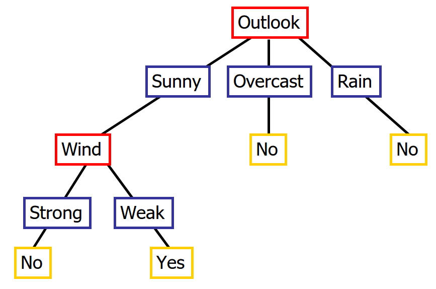
Decision Tree using Conjunction (AND Operation)
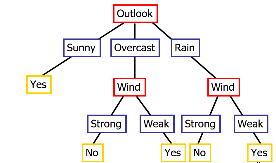
Decision Tree using Disjunction (OR Operations)
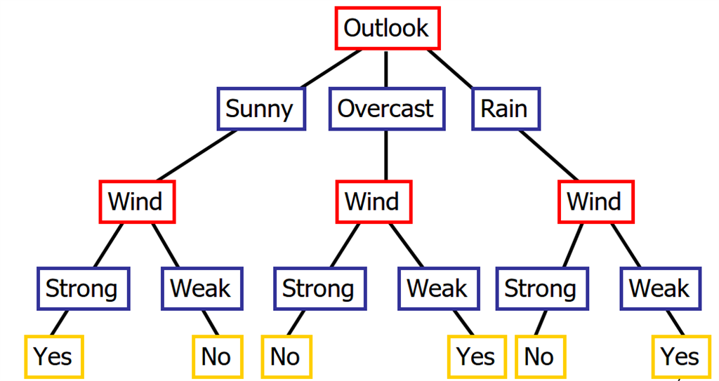
Decision Tree using XOR
Decision Tree using Disjunction of Conjunctions (OR of AND Operations)
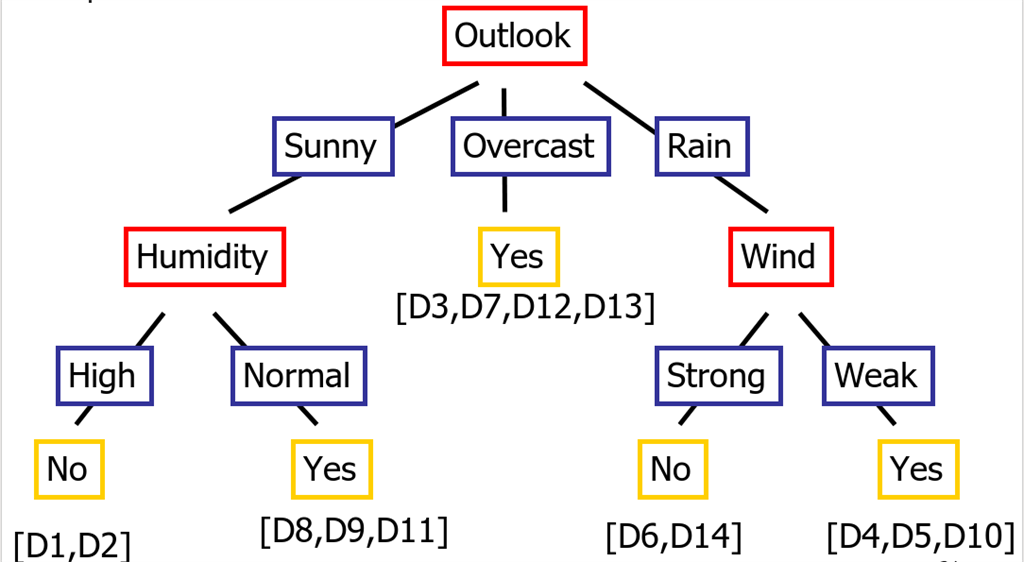
Let us look at a rough decision tree, to look at how exactly the decision tree will look like
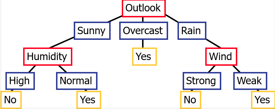
From the above trees we aren't able to clearly infer anything, so let me show you how exactly the Decision Tree will look for the given dataset, and then we will try to understand, what exactly that tree means and how to use the tree to our benefit.
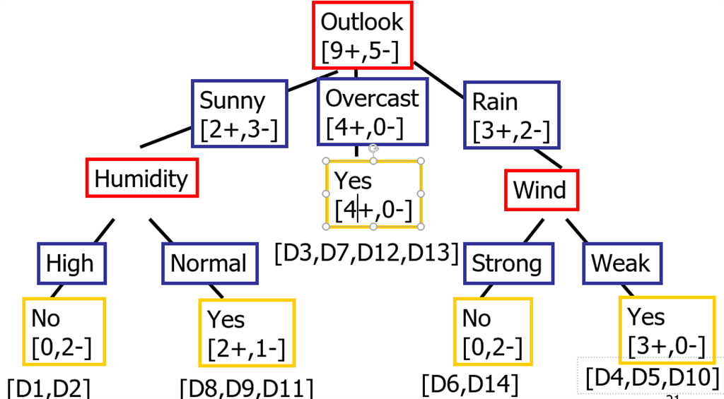
You may be wondering why did we take "Outlook" as root node", it is
because of the Gini Index value, calculated earlier
Following is the Decision Tree with the Weights which can be used to calculate entropy and information gain.
Now let's try to understand the tree,
R1: If (Outlook=Sunny) _| (Humidity=High) Then PlayTennis=No
The above statement means that if Outlook is Sunny and Humidity is high, then we do not play
R2: If (Outlook=Sunny) _| (Humidity=Normal) Then PlayTennis=Yes
The above statement means that if Outlook is Sunny and Humidity is normal, then we play
R3: If (Outlook=Overcast) Then PlayTennis=Yes
The above statement means that if Outlook is Overcast, then we play
R4: If (Outlook=Rain) -| (Wind=Strong) Then PlayTennis=Yes
The above statement means that if Outlook is Rain or Wild is Strong, then we play
Python Implementation of Decision Tree
Let's take the example of the IRIS dataset, you can directly import it from the sklearn dataset repository. Feel free to use any dataset,
there some very good datasets available on kaggle and with Google Colab.
The dataset that I will be using here is UCI Zoo Dataset.
1. Using NumPy
- import pandas as pd
- import numpy as np
- from pprint import pprint
- #Import the dataset and define the feature as well as the target datasets / columns#
- dataset = pd.read_csv('zoo.csv',
- names=['animal_name','hair','feathers','eggs','milk',
- 'airbone','aquatic','predator','toothed','backbone',
- 'breathes','venomous','fins','legs','tail','domestic','catsize','class',])#Import all columns omitting the fist which consists the names of the animals
- #We drop the animal names since this is not a good feature to split the data on
- dataset=dataset.drop('animal_name',axis=1)
- def entropy(target_col):
- elements,counts = np.unique(target_col,return_counts = True)
- entropy = np.sum([(-counts[i]/np.sum(counts))*np.log2(counts[i]/np.sum(counts)) for i in range(len(elements))])
- return entropy
- def InfoGain(data,split_attribute_name,target_name="class"):
- #Calculate the entropy of the total dataset
- total_entropy = entropy(data[target_name])
- ##Calculate the entropy of the dataset
- #Calculate the values and the corresponding counts for the split attribute
- vals,counts= np.unique(data[split_attribute_name],return_counts=True)
- #Calculate the weighted entropy
- Weighted_Entropy = np.sum([(counts[i]/np.sum(counts))*entropy(data.where(data[split_attribute_name]==vals[i]).dropna()[target_name]) for i in range(len(vals))])
- #Calculate the information gain
- Information_Gain = total_entropy - Weighted_Entropy
- return Information_Gain
- def ID3(data,originaldata,features,target_attribute_name="class",parent_node_class = None):
- #Define the stopping criteria --> If one of this is satisfied, we want to return a leaf node#
- #If all target_values have the same value, return this value
- if len(np.unique(data[target_attribute_name])) <= 1:
- return np.unique(data[target_attribute_name])[0]
- #If the dataset is empty, return the mode target feature value in the original dataset
- elif len(data)==0:
- return np.unique(originaldata[target_attribute_name])[np.argmax(np.unique(originaldata[target_attribute_name],return_counts=True)[1])]
- #If the feature space is empty, return the mode target feature value of the direct parent node --> Note that
- #the direct parent node is that node which has called the current run of the ID3 algorithm and hence
- #the mode target feature value is stored in the parent_node_class variable.
- elif len(features) ==0:
- return parent_node_class
- #If none of the above holds true, grow the tree!
- else:
- #Set the default value for this node --> The mode target feature value of the current node
- parent_node_class = np.unique(data[target_attribute_name])[np.argmax(np.unique(data[target_attribute_name],return_counts=True)[1])]
- #Select the feature which best splits the dataset
- item_values = [InfoGain(data,feature,target_attribute_name) for feature in features] #Return the information gain values for the features in the dataset
- best_feature_index = np.argmax(item_values)
- best_feature = features[best_feature_index]
- #Create the tree structure. The root gets the name of the feature (best_feature) with the maximum information
- #gain in the first run
- tree = {best_feature:{}}
- #Remove the feature with the best inforamtion gain from the feature space
- features = [i for i in features if i != best_feature]
- #Grow a branch under the root node for each possible value of the root node feature
- for value in np.unique(data[best_feature]):
- value = value
- #Split the dataset along the value of the feature with the largest information gain and therwith create sub_datasets
- sub_data = data.where(data[best_feature] == value).dropna()
- #Call the ID3 algorithm for each of those sub_datasets with the new parameters --> Here the recursion comes in!
- subtree = ID3(sub_data,dataset,features,target_attribute_name,parent_node_class)
- #Add the sub tree, grown from the sub_dataset to the tree under the root node
- tree[best_feature][value] = subtree
- return(tree)
- def predict(query,tree,default = 1):
- for key in list(query.keys()):
- if key in list(tree.keys()):
- try:
- result = tree[key][query[key]]
- except:
- return default
- result = tree[key][query[key]]
- if isinstance(result,dict):
- return predict(query,result)
- else:
- return result
- def train_test_split(dataset):
- training_data = dataset.iloc[:80].reset_index(drop=True)#We drop the index respectively relabel the index
- #starting form 0, because we do not want to run into errors regarding the row labels / indexes
- testing_data = dataset.iloc[80:].reset_index(drop=True)
- return training_data,testing_data
- training_data = train_test_split(dataset)[0]
- testing_data = train_test_split(dataset)[1]
- def test(data,tree):
- #Create new query instances by simply removing the target feature column from the original dataset and
- #convert it to a dictionary
- queries = data.iloc[:,:-1].to_dict(orient = "records")
- #Create a empty DataFrame in whose columns the prediction of the tree are stored
- predicted = pd.DataFrame(columns=["predicted"])
- #Calculate the prediction accuracy
- for i in range(len(data)):
- predicted.loc[i,"predicted"] = predict(queries[i],tree,1.0)
- print('The prediction accuracy is: ',(np.sum(predicted["predicted"] == data["class"])/len(data))*100,'%')
- tree = ID3(training_data,training_data,training_data.columns[:-1])
- pprint(tree)
- test(testing_data,tree)
the output that I got is
{'legs': {0: {'fins': {0.0: {'toothed': {0.0: 7.0, 1.0: 3.0}},
1.0: {'eggs': {0.0: 1.0, 1.0: 4.0}}}},
2: {'hair': {0.0: 2.0, 1.0: 1.0}},
4: {'hair': {0.0: {'toothed': {0.0: 7.0, 1.0: 5.0}}, 1.0: 1.0}},
6: {'aquatic': {0.0: 6.0, 1.0: 7.0}}, 8: 7.0}}
The prediction accuracy is: 85.71428571428571 %
2. Using SKLearn
- #Import the DecisionTreeClassifier
- from sklearn.tree import DecisionTreeClassifier
- #Import the dataset
- dataset = pd.read_csv('zoo.csv',
- names=['animal_name','hair','feathers','eggs','milk',
- 'airbone','aquatic','predator','toothed','backbone',
- 'breathes','venomous','fins','legs','tail','domestic','catsize','class',])
- #We drop the animal names since this is not a good feature to split the data on
- dataset=dataset.drop('animal_name',axis=1)
- train_features = dataset.iloc[:80,:-1]
- test_features = dataset.iloc[80:,:-1]
- train_targets = dataset.iloc[:80,-1]
- test_targets = dataset.iloc[80:,-1]
- tree = DecisionTreeClassifier(criterion = 'entropy').fit(train_features,train_targets)
- prediction = tree.predict(test_features)
- print("The prediction accuracy is: ",tree.score(test_features,test_targets)*100,"%")
The output that I got is:
The prediction accuracy is: 80.95238095238095 %
3. Using TensorFlow
- import numpy as np
- import pandas as pd
- import tensorflow as tf
- from functools import reduce
- import matplotlib.pyplot as plt
- %matplotlib inline
- np.random.seed(1943)
- tf.set_random_seed(1943)
- iris = [((5.1, 3.5, 1.4, 0.2), (1, 0, 0)),
- ((4.9, 3.0, 1.4, 0.2), (1, 0, 0)),
- ((4.7, 3.2, 1.3, 0.2), (1, 0, 0)),
- ((4.6, 3.1, 1.5, 0.2), (1, 0, 0)),
- ((5.0, 3.6, 1.4, 0.2), (1, 0, 0)),
- ((5.4, 3.9, 1.7, 0.4), (1, 0, 0)),
- ((4.6, 3.4, 1.4, 0.3), (1, 0, 0)),
- ((5.0, 3.4, 1.5, 0.2), (1, 0, 0)),
- ((4.4, 2.9, 1.4, 0.2), (1, 0, 0)),
- ((4.9, 3.1, 1.5, 0.1), (1, 0, 0)),
- ((5.4, 3.7, 1.5, 0.2), (1, 0, 0)),
- ((4.8, 3.4, 1.6, 0.2), (1, 0, 0)),
- ((4.8, 3.0, 1.4, 0.1), (1, 0, 0)),
- ((4.3, 3.0, 1.1, 0.1), (1, 0, 0)),
- ((5.8, 4.0, 1.2, 0.2), (1, 0, 0)),
- ((5.7, 4.4, 1.5, 0.4), (1, 0, 0)),
- ((5.4, 3.9, 1.3, 0.4), (1, 0, 0)),
- ((5.1, 3.5, 1.4, 0.3), (1, 0, 0)),
- ((5.7, 3.8, 1.7, 0.3), (1, 0, 0)),
- ((5.1, 3.8, 1.5, 0.3), (1, 0, 0)),
- ((5.4, 3.4, 1.7, 0.2), (1, 0, 0)),
- ((5.1, 3.7, 1.5, 0.4), (1, 0, 0)),
- ((4.6, 3.6, 1.0, 0.2), (1, 0, 0)),
- ((5.1, 3.3, 1.7, 0.5), (1, 0, 0)),
- ((4.8, 3.4, 1.9, 0.2), (1, 0, 0)),
- ((5.0, 3.0, 1.6, 0.2), (1, 0, 0)),
- ((5.0, 3.4, 1.6, 0.4), (1, 0, 0)),
- ((5.2, 3.5, 1.5, 0.2), (1, 0, 0)),
- ((5.2, 3.4, 1.4, 0.2), (1, 0, 0)),
- ((4.7, 3.2, 1.6, 0.2), (1, 0, 0)),
- ((4.8, 3.1, 1.6, 0.2), (1, 0, 0)),
- ((5.4, 3.4, 1.5, 0.4), (1, 0, 0)),
- ((5.2, 4.1, 1.5, 0.1), (1, 0, 0)),
- ((5.5, 4.2, 1.4, 0.2), (1, 0, 0)),
- ((4.9, 3.1, 1.5, 0.1), (1, 0, 0)),
- ((5.0, 3.2, 1.2, 0.2), (1, 0, 0)),
- ((5.5, 3.5, 1.3, 0.2), (1, 0, 0)),
- ((4.9, 3.1, 1.5, 0.1), (1, 0, 0)),
- ((4.4, 3.0, 1.3, 0.2), (1, 0, 0)),
- ((5.1, 3.4, 1.5, 0.2), (1, 0, 0)),
- ((5.0, 3.5, 1.3, 0.3), (1, 0, 0)),
- ((4.5, 2.3, 1.3, 0.3), (1, 0, 0)),
- ((4.4, 3.2, 1.3, 0.2), (1, 0, 0)),
- ((5.0, 3.5, 1.6, 0.6), (1, 0, 0)),
- ((5.1, 3.8, 1.9, 0.4), (1, 0, 0)),
- ((4.8, 3.0, 1.4, 0.3), (1, 0, 0)),
- ((5.1, 3.8, 1.6, 0.2), (1, 0, 0)),
- ((4.6, 3.2, 1.4, 0.2), (1, 0, 0)),
- ((5.3, 3.7, 1.5, 0.2), (1, 0, 0)),
- ((5.0, 3.3, 1.4, 0.2), (1, 0, 0)),
- ((7.0, 3.2, 4.7, 1.4), (0, 1, 0)),
- ((6.4, 3.2, 4.5, 1.5), (0, 1, 0)),
- ((6.9, 3.1, 4.9, 1.5), (0, 1, 0)),
- ((5.5, 2.3, 4.0, 1.3), (0, 1, 0)),
- ((6.5, 2.8, 4.6, 1.5), (0, 1, 0)),
- ((5.7, 2.8, 4.5, 1.3), (0, 1, 0)),
- ((6.3, 3.3, 4.7, 1.6), (0, 1, 0)),
- ((4.9, 2.4, 3.3, 1.0), (0, 1, 0)),
- ((6.6, 2.9, 4.6, 1.3), (0, 1, 0)),
- ((5.2, 2.7, 3.9, 1.4), (0, 1, 0)),
- ((5.0, 2.0, 3.5, 1.0), (0, 1, 0)),
- ((5.9, 3.0, 4.2, 1.5), (0, 1, 0)),
- ((6.0, 2.2, 4.0, 1.0), (0, 1, 0)),
- ((6.1, 2.9, 4.7, 1.4), (0, 1, 0)),
- ((5.6, 2.9, 3.6, 1.3), (0, 1, 0)),
- ((6.7, 3.1, 4.4, 1.4), (0, 1, 0)),
- ((5.6, 3.0, 4.5, 1.5), (0, 1, 0)),
- ((5.8, 2.7, 4.1, 1.0), (0, 1, 0)),
- ((6.2, 2.2, 4.5, 1.5), (0, 1, 0)),
- ((5.6, 2.5, 3.9, 1.1), (0, 1, 0)),
- ((5.9, 3.2, 4.8, 1.8), (0, 1, 0)),
- ((6.1, 2.8, 4.0, 1.3), (0, 1, 0)),
- ((6.3, 2.5, 4.9, 1.5), (0, 1, 0)),
- ((6.1, 2.8, 4.7, 1.2), (0, 1, 0)),
- ((6.4, 2.9, 4.3, 1.3), (0, 1, 0)),
- ((6.6, 3.0, 4.4, 1.4), (0, 1, 0)),
- ((6.8, 2.8, 4.8, 1.4), (0, 1, 0)),
- ((6.7, 3.0, 5.0, 1.7), (0, 1, 0)),
- ((6.0, 2.9, 4.5, 1.5), (0, 1, 0)),
- ((5.7, 2.6, 3.5, 1.0), (0, 1, 0)),
- ((5.5, 2.4, 3.8, 1.1), (0, 1, 0)),
- ((5.5, 2.4, 3.7, 1.0), (0, 1, 0)),
- ((5.8, 2.7, 3.9, 1.2), (0, 1, 0)),
- ((6.0, 2.7, 5.1, 1.6), (0, 1, 0)),
- ((5.4, 3.0, 4.5, 1.5), (0, 1, 0)),
- ((6.0, 3.4, 4.5, 1.6), (0, 1, 0)),
- ((6.7, 3.1, 4.7, 1.5), (0, 1, 0)),
- ((6.3, 2.3, 4.4, 1.3), (0, 1, 0)),
- ((5.6, 3.0, 4.1, 1.3), (0, 1, 0)),
- ((5.5, 2.5, 4.0, 1.3), (0, 1, 0)),
- ((5.5, 2.6, 4.4, 1.2), (0, 1, 0)),
- ((6.1, 3.0, 4.6, 1.4), (0, 1, 0)),
- ((5.8, 2.6, 4.0, 1.2), (0, 1, 0)),
- ((5.0, 2.3, 3.3, 1.0), (0, 1, 0)),
- ((5.6, 2.7, 4.2, 1.3), (0, 1, 0)),
- ((5.7, 3.0, 4.2, 1.2), (0, 1, 0)),
- ((5.7, 2.9, 4.2, 1.3), (0, 1, 0)),
- ((6.2, 2.9, 4.3, 1.3), (0, 1, 0)),
- ((5.1, 2.5, 3.0, 1.1), (0, 1, 0)),
- ((5.7, 2.8, 4.1, 1.3), (0, 1, 0)),
- ((6.3, 3.3, 6.0, 2.5), (0, 0, 1)),
- ((5.8, 2.7, 5.1, 1.9), (0, 0, 1)),
- ((7.1, 3.0, 5.9, 2.1), (0, 0, 1)),
- ((6.3, 2.9, 5.6, 1.8), (0, 0, 1)),
- ((6.5, 3.0, 5.8, 2.2), (0, 0, 1)),
- ((7.6, 3.0, 6.6, 2.1), (0, 0, 1)),
- ((4.9, 2.5, 4.5, 1.7), (0, 0, 1)),
- ((7.3, 2.9, 6.3, 1.8), (0, 0, 1)),
- ((6.7, 2.5, 5.8, 1.8), (0, 0, 1)),
- ((7.2, 3.6, 6.1, 2.5), (0, 0, 1)),
- ((6.5, 3.2, 5.1, 2.0), (0, 0, 1)),
- ((6.4, 2.7, 5.3, 1.9), (0, 0, 1)),
- ((6.8, 3.0, 5.5, 2.1), (0, 0, 1)),
- ((5.7, 2.5, 5.0, 2.0), (0, 0, 1)),
- ((5.8, 2.8, 5.1, 2.4), (0, 0, 1)),
- ((6.4, 3.2, 5.3, 2.3), (0, 0, 1)),
- ((6.5, 3.0, 5.5, 1.8), (0, 0, 1)),
- ((7.7, 3.8, 6.7, 2.2), (0, 0, 1)),
- ((7.7, 2.6, 6.9, 2.3), (0, 0, 1)),
- ((6.0, 2.2, 5.0, 1.5), (0, 0, 1)),
- ((6.9, 3.2, 5.7, 2.3), (0, 0, 1)),
- ((5.6, 2.8, 4.9, 2.0), (0, 0, 1)),
- ((7.7, 2.8, 6.7, 2.0), (0, 0, 1)),
- ((6.3, 2.7, 4.9, 1.8), (0, 0, 1)),
- ((6.7, 3.3, 5.7, 2.1), (0, 0, 1)),
- ((7.2, 3.2, 6.0, 1.8), (0, 0, 1)),
- ((6.2, 2.8, 4.8, 1.8), (0, 0, 1)),
- ((6.1, 3.0, 4.9, 1.8), (0, 0, 1)),
- ((6.4, 2.8, 5.6, 2.1), (0, 0, 1)),
- ((7.2, 3.0, 5.8, 1.6), (0, 0, 1)),
- ((7.4, 2.8, 6.1, 1.9), (0, 0, 1)),
- ((7.9, 3.8, 6.4, 2.0), (0, 0, 1)),
- ((6.4, 2.8, 5.6, 2.2), (0, 0, 1)),
- ((6.3, 2.8, 5.1, 1.5), (0, 0, 1)),
- ((6.1, 2.6, 5.6, 1.4), (0, 0, 1)),
- ((7.7, 3.0, 6.1, 2.3), (0, 0, 1)),
- ((6.3, 3.4, 5.6, 2.4), (0, 0, 1)),
- ((6.4, 3.1, 5.5, 1.8), (0, 0, 1)),
- ((6.0, 3.0, 4.8, 1.8), (0, 0, 1)),
- ((6.9, 3.1, 5.4, 2.1), (0, 0, 1)),
- ((6.7, 3.1, 5.6, 2.4), (0, 0, 1)),
- ((6.9, 3.1, 5.1, 2.3), (0, 0, 1)),
- ((5.8, 2.7, 5.1, 1.9), (0, 0, 1)),
- ((6.8, 3.2, 5.9, 2.3), (0, 0, 1)),
- ((6.7, 3.3, 5.7, 2.5), (0, 0, 1)),
- ((6.7, 3.0, 5.2, 2.3), (0, 0, 1)),
- ((6.3, 2.5, 5.0, 1.9), (0, 0, 1)),
- ((6.5, 3.0, 5.2, 2.0), (0, 0, 1)),
- ((6.2, 3.4, 5.4, 2.3), (0, 0, 1)),
- ((5.9, 3.0, 5.1, 1.8), (0, 0, 1))]
- feature = np.vstack([np.array(i[0]) for i in iris])
- label = np.vstack([np.array(i[1]) for i in iris])
- x = feature[:, 2:4] # use "Petal length" and "Petal width" only
- y = label
- d = x.shape[1]
- def tf_kron_prod(a, b):
- res = tf.einsum('ij,ik->ijk', a, b)
- res = tf.reshape(res, [-1, tf.reduce_prod(res.shape[1:])])
- return res
- def tf_bin(x, cut_points, temperature=0.1):
- # x is a N-by-1 matrix (column vector)
- # cut_points is a D-dim vector (D is the number of cut-points)
- # this function produces a N-by-(D+1) matrix, each row has only one element being one and the rest are all zeros
- D = cut_points.get_shape().as_list()[0]
- W = tf.reshape(tf.linspace(1.0, D + 1.0, D + 1), [1, -1])
- cut_points = tf.contrib.framework.sort(cut_points) # make sure cut_points is monotonically increasing
- b = tf.cumsum(tf.concat([tf.constant(0.0, shape=[1]), -cut_points], 0))
- h = tf.matmul(x, W) + b
- res = tf.nn.softmax(h / temperature)
- return res
- def nn_decision_tree(x, cut_points_list, leaf_score, temperature=0.1):
- # cut_points_list contains the cut_points for each dimension of feature
- leaf = reduce(tf_kron_prod,
- map(lambda z: tf_bin(x[:, z[0]:z[0] + 1], z[1], temperature), enumerate(cut_points_list)))
- return tf.matmul(leaf, leaf_score)
- num_cut = [1, 1] # "Petal length" and "Petal width"
- num_leaf = np.prod(np.array(num_cut) + 1)
- num_class = 3
- sess = tf.InteractiveSession()
- x_ph = tf.placeholder(tf.float32, [None, d])
- y_ph = tf.placeholder(tf.float32, [None, num_class])
- cut_points_list = [tf.Variable(tf.random_uniform([i])) for i in num_cut]
- leaf_score = tf.Variable(tf.random_uniform([num_leaf, num_class]))
- y_pred = nn_decision_tree(x_ph, cut_points_list, leaf_score, temperature=0.1)
- loss = tf.reduce_mean(tf.losses.softmax_cross_entropy(logits=y_pred, onehot_labels=y_ph))
- opt = tf.train.AdamOptimizer(0.1)
- train_step = opt.minimize(loss)
- sess.run(tf.global_variables_initializer())
- for i in range(1000):
- _, loss_e = sess.run([train_step, loss], feed_dict={x_ph: x, y_ph: y})
- if i % 200 == 0:
- print(loss_e)
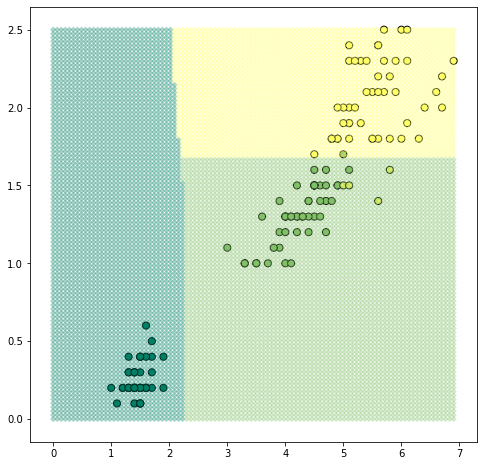
- print('error rate %.2f' % (1 - np.mean(np.argmax(y_pred.eval(feed_dict={x_ph: x}), axis=1) == np.argmax(y, axis=1))))
- sample_x0 = np.repeat(np.linspace(0, np.max(x[:,0]), 100), 100).reshape(-1,1)
- sample_x1 = np.tile(np.linspace(0, np.max(x[:,1]), 100).reshape(-1,1), [100,1])
- sample_x = np.hstack([sample_x0, sample_x1])
- sample_label = np.argmax(y_pred.eval(feed_dict={x_ph: sample_x}), axis=1)
- plt.figure(figsize=(8,8))
- plt.scatter(x[:,0],
- x[:,1],
- c=np.argmax(y, axis=1),
- marker='o',
- s=50,
- cmap='summer',
- edgecolors='black')
- plt.scatter(sample_x0.flatten(),
- sample_x1.flatten(),
- c=sample_label.flatten(),
- marker='D',
- s=20,
- cmap='summer',
- edgecolors='none',
- alpha=0.33)
1.1529802
0.32481167
0.1562062
0.15097024
0.118773825
error rate 0.04
Conclusion
In this chapter, we studied about decision tree.
In the next chapter, we will study about Naive Bayes.
Author

Rohit Gupta
13
61k
3.2m